[SQL튜닝]23.11.20

망구씨·2023년 11월 20일

SQL 튜닝

목록 보기

7/9

db 엔지니어 또는 dba로 일할 때 필요한 스크립트 이번주에 모으기
대기 이벤트 보면서 원인 파악
간단한 SQL 튜닝

복습! SQL튜닝

1. table access 방법

  * 전체 테이블 스캔 : /*+ full(테이블명) */
  * rowid에 의한 스캔 : /*+ rowid */
  * sample 스캔 (따로 힌트는 없다.)

2. index access 방법

  * index range scan  : /*+ index(테이블명 인덱스명) */ 
  * index unique scan : /*+ index(테이블명 인덱스명) */
  * index full scan : /*+ index_fs(테이블명 인덱스명) */
  * index fast full scan : /*+ index_ffs(테이블명 인덱스명) */
  * index skip scan : /*+ index_ss(테이블명 인덱스명) */
  * index merge scan : /*+ and_equal(테이블 인덱스명1 인덱스명2) */ 
  * index bitmap merge scan : /*+ index_combine(테이블명) */ 
  * index join  : /*+ index_join(테이블명 인덱스명1 인덱스명2) */

✔️ index join scan 방법

💡 인덱스 끼리 조인을 해서 테이블 엑세스를 따로 하지 않는 스캔 방식!
/*+ index_join(테이블명 인덱스명1 인덱스명2) */

실습

@demo
create index emp_deptno on emp(deptno);
create index emp_job on emp(job);

select /*+ gather_plan_statistics index_join(emp emp_deptno emp_job) */ deptno, job
  from emp
  where deptno = 30 and job = 'SALESMAN';

 ----------------------------------------------------------------------------------------------------------------------------
| Id  | Operation          | Name             | Starts | E-Rows | A-Rows |   A-Time   | Buffers |  OMem |  1Mem | Used-Mem |
----------------------------------------------------------------------------------------------------------------------------
|   0 | SELECT STATEMENT   |                  |      1 |        |      4 |00:00:00.01 |       2 |       |       |          |
|*  1 |  VIEW              | index$_join$_001 |      1 |      4 |      4 |00:00:00.01 |       2 |       |       |          |
|*  2 |   HASH JOIN        |                  |      1 |        |      4 |00:00:00.01 |       2 |  1519K|  1519K| 1093K (0)|
|*  3 |    INDEX RANGE SCAN| EMP_DEPTNO       |      1 |      4 |      6 |00:00:00.01 |       1 |       |       |          |
|*  4 |    INDEX RANGE SCAN| EMP_JOB          |      1 |      4 |      4 |00:00:00.01 |       1 |       |       |          |
----------------------------------------------------------------------------------------------------------------------------

➡️ 인덱스에 이미 deptno, job이 있으므로 테이블 엑세스를 하지 않고 그냥 2개의 인덱스를 조인한 것!!

문제1. 아래의 환경을 만들기

drop table sales600 purge;
create table sales600
as
 select * from sh.sales;
 
create index sales600_indx1 on sales600(channel_id);
create index sales600_indx2 on sales600(prod_id);

문제2. sales600에서 channel_id가 3 이고, prod_id가 144인 데이터의 channel_id와 prod_id를 쿼리하는 SQL을 index join실행계획으로 출력하기

select /*+ gather_plan_statistics index_join(sales600 sales600_indx1 sales600_indx2) */ channel_id, prod_id
  from sales600
  where channel_id=3 and prod_id=144;
 
SELECT * 
FROM TABLE(dbms_xplan.display_cursor(null,null,'ALLSTATS LAST'));

➡️ 버퍼의 갯수 1275개!

문제3. channel_id, prod_id를 결합 컬럼 인덱스로 생성하기 결합 컬럼 인덱스의 이름은 sales600_indx3

create index sales600_indx3
  on sales600(channel_id,prod_id);

문제4. 아래의 쿼리문이 sales600_indx3 인덱스를 엑세스 하도록 힌트르 주고 실행하면 버퍼의 갯수가 몇개인지 확인하기!

select /*+ gather_plan_statistics index(sales600 sales600_indx3) */ channel_id, prod_id
  from sales600
  where channel_id=3 and prod_id=144;

SELECT * 
FROM TABLE(dbms_xplan.display_cursor(null,null,'ALLSTATS LAST'));

➡️ 버퍼의 갯수가 213개로 줄어들었다!

💡 인덱스 조인보다 결합 컬럼 인덱스가 훨씬 더 튜닝 SQL이다!

✍🏻 인덱스 관련한 추가 튜닝 내용 1 (결합 컬럼 인덱스의 컬럼 구성 순서의 중요성)

아래의 두개의 인덱스 중 어느 인덱스가 더 좋은 인덱스인가? prod_id가 선두 컬럼에 있을때와 channel_id가 선두컬럼에 있을 때!!

drop table sales600 purge;
create table sales600
as
 select * from sh.sales;

create index sales600_indx1 on sales600(prod_id, channel_id);
create index sales600_indx2 on sales600(channel_id, prod_id);

문제1. 힌트를 주고 위 두개의 인덱스를 각각 엑세스 해서 어느 인덱스가 더 버퍼의 갯수가 작은지

-- sales600_indx1 사용 : 버퍼의 갯수 457개
select /*+ gather_plan_statistics index(sales600 sales600_indx1) */ *
 from sales600
 where channel_id=3 and prod_id=144;

-- sales600_indx2 사용 : 버퍼의 갯수 456개
select /*+ gather_plan_statistics index(sales600 sales600_indx2) */ *
 from sales600
 where channel_id=3 and prod_id=144;

SELECT * 
FROM TABLE(dbms_xplan.display_cursor(null,null,'ALLSTATS LAST')); 
➡️ 버퍼의 갯수가 차이가 없어서 똑같다고 보면 되지만, 결합 컬럼 인덱스를 생성할 때 컬럼 구성은 앞에 있는 컬럼이 선택도가 좋은 컬럼을 앞으로 두어야 한다.
# ex)
create index emp_indx1 on emp(job,deptno);
create index emp_indx2 on emp(deptno,job);

select /*+ gather_plan_statistics */ * 
 from emp
 where job='PRESIDENT' and deptno = 10; 
➡️ 직업은 14명중 1명이 있고 deptno는 14명중 3명이 있다. 직업이 선택도가 더 좋다. 위 쿼리문을 실행하면 옵티마이저가 emp_indx1를 탄다.

⭐ 튜닝 tip !

select /*+ gather_plan_statistics index(emp emp_indx1) */ * 
 from emp
 where 1=1
   and job='PRESIDENT'  -- 1건
   and deptno = 10;     -- 3건

➡️ count해서 몇개가 있는지 다 찾아본 후에 튜닝을 한다!
➡️ sqldeveloper에서 테이블 클릭>인덱스 에서 인덱스 정보를 확인한다. 어떤 컬럼이 앞에 있는지 볼 수 있음!! 혹은 아래처럼

💡 결합 컬럼 인덱스의 컬럼 순서 확인하는 방법!
select index_name, column_name, column_position
  from user_ind_columns
  where table_name='EMP';

✍🏻 인덱스 관련한 추가 튜닝 내용 2 (결합 컬럼 인덱스의 컬럼 구성 순서의 중요성2)

환경 구성

create table 월별고객별판매집계
as
select rownum 고객번호
     , '2008' || lpad(ceil(rownum/100000), 2, '0') 판매월
     , decode(mod(rownum, 12), 1, 'A', 'B') 판매구분
     , round(dbms_random.value(1000,100000), -2) 판매금액
from   dual
connect by level <= 1200000 ;

create index m_IDX1 on 월별고객별판매집계(판매구분, 판매월);
create index m_IDX2 on 월별고객별판매집계(판매월, 판매구분);

❓ 옵티마이저는 아래의 SQL에서 위 2개의 인덱스중에 어느 인덱스를 엑세스 할까??

select /*+ gather_plan_statistics*/ count(*)
from   월별고객별판매집계 t
where  판매구분 = 'A' # ★ 점조건 
and    판매월 between '200801' and '200812'; # ★ 선분조건

SELECT * 
FROM TABLE(dbms_xplan.display_cursor(null,null,'ALLSTATS LAST')); 

--------------------------------------------------------------------------------------
| Id  | Operation         | Name   | Starts | E-Rows | A-Rows |   A-Time   | Buffers |
--------------------------------------------------------------------------------------
|   0 | SELECT STATEMENT  |        |      1 |        |      1 |00:00:00.01 |     281 |
|   1 |  SORT AGGREGATE   |        |      1 |      1 |      1 |00:00:00.01 |     281 |
|*  2 |   INDEX RANGE SCAN| M_IDX1 |      1 |    102K|    100K|00:00:00.01 |     281 |
--------------------------------------------------------------------------------------
# 버퍼 갯수 281개!

➡️ M_IDX1 인덱스를 탔다! 선택도가 판매구분이 더 좋기도 하지만 where절에 이퀄(=)조건의 컬럼이 결합 컬럼 인덱스의 선두 컬럼에 있어야 더 좋은 성능을 보인다!

점조건 : =이나 in을 사용한 조건
선분 조건 :beteen..and 나 like를 사용한 조건

💡 결합 컬럼 인덱스를 구성할 때는 점조건이 선두 컬럼으로 구성되는것이 바람직하다! 인덱스를 생성하기 전에 이 인덱스가 필요한 SQL들을 조사해서 점조건이 있는 컬럼을 선두 컬럼으로 구성을 해야 한다.

문제1. 아래 SQL이 m_dix2 인덱스를 엑세스 했을 때 버퍼의 갯수 확인해보기

select /*+ gather_plan_statistics index(t m_IDX2) */ count(*)
from   월별고객별판매집계 t
where  판매구분 = 'A' 
and    판매월 between '200801' and '200812'; 

-----------------------------------------------------------------------------------------------
| Id  | Operation         | Name   | Starts | E-Rows | A-Rows |   A-Time   | Buffers | Reads  |
-----------------------------------------------------------------------------------------------
|   0 | SELECT STATEMENT  |        |      1 |        |      1 |00:00:00.50 |    3090 |   3100 |
|   1 |  SORT AGGREGATE   |        |      1 |      1 |      1 |00:00:00.50 |    3090 |   3100 |
|*  2 |   INDEX RANGE SCAN| M_IDX2 |      1 |    102K|    100K|00:00:00.09 |    3090 |   3100 |
-----------------------------------------------------------------------------------------------

➡️ 버퍼의 갯수가 m_IDX1을 엑세스 했을 때는 281개 였지만 M_IDX2를 엑세스 하니 3100개로 늘어났다!

❓ 그런데 인덱스가 m_IDX2 밖에 없는 상황이라면? -> 판매월이 선두컬럼으로 있는 인덱스!

drop index m_IDX1;

m_IDX2 를 엑세스 하자니 버퍼의 갯수가 3100이나 되었다. 그렇다면 full table scan의 버퍼의 갯수 확인해보기

select /*+ gather_plan_statistics full(t) */ count(*)
from   월별고객별판매집계 t
where  판매구분 = 'A' 
and    판매월 between '200801' and '200812';   

---------------------------------------------------------------------------------------------------
| Id  | Operation          | Name      | Starts | E-Rows | A-Rows |   A-Time   | Buffers | Reads  |
---------------------------------------------------------------------------------------------------
|   0 | SELECT STATEMENT   |           |      1 |        |      1 |00:00:00.24 |    3832 |   3829 |
|   1 |  SORT AGGREGATE    |           |      1 |      1 |      1 |00:00:00.24 |    3832 |   3829 |
|*  2 |   TABLE ACCESS FULL| 월별고객별|      1 |    102K|    100K|00:00:00.06 |    3832 |   3829 |
---------------------------------------------------------------------------------------------------

➡️ 버퍼의 갯수가 3832개 이다.

💡 SQL을 재작성해서 튜닝하는 방법?

1. 튜닝전 (m_indx2 엑세스)

select /*+ gather_plan_statistics index(t m_IDX2) */ count(*)
from   월별고객별판매집계 t
where  판매구분 = 'A' 
and    판매월 between '200801' and '200812';

------------------------------------------------------------------------------------------
| Id  | Operation             | Name   | Starts | E-Rows | A-Rows |   A-Time   | Buffers |
------------------------------------------------------------------------------------------
|   0 | SELECT STATEMENT      |        |      1 |        |      1 |00:00:00.04 |    3366 |
|   1 |  SORT AGGREGATE       |        |      1 |      1 |      1 |00:00:00.04 |    3366 |
|*  2 |   INDEX FAST FULL SCAN| M_IDX2 |      1 |    102K|    100K|00:00:00.01 |    3366 |
------------------------------------------------------------------------------------------

2. 판매월 between '200801' and '200812' 이 선분조건을 점조건으로 변경해주기

-- 튜닝 전 코드임
select /*+ gather_plan_statistics index(t m_IDX2) */ count(*)
from   월별고객별판매집계 t
where  판매구분 = 'A' 
and    판매월 between '200801' and '200812';

3. where절을 점조건으로 바꿔주기 위해 확인하기 (in을 써야한다.)

select distinct 판매월 
 from 월별고객별판매집계
 where 판매월 between '200801' and '200812'
 order by 1 asc;
---------------------------------
200801
200802
200803
200804
200805
200806
200807
200808
200809
200810
200811
200812

4. 튜닝 후 (SQL튜닝)

select /*+ gather_plan_statistics index(t m_IDX2) */ count(*)
from   월별고객별판매집계 t
where  판매구분 = 'A' 
and    판매월 in ( '200801', '200802', '200803', '200804', '200805', '200806', '200807', '200808', '200809', '200810', '200811', '200812')

---------------------------------------------------------------------------------------
| Id  | Operation          | Name   | Starts | E-Rows | A-Rows |   A-Time   | Buffers |
---------------------------------------------------------------------------------------
|   0 | SELECT STATEMENT   |        |      1 |        |      1 |00:00:00.01 |     304 |
|   1 |  SORT AGGREGATE    |        |      1 |      1 |      1 |00:00:00.01 |     304 |
|   2 |   INLIST ITERATOR  |        |      1 |        |    100K|00:00:00.02 |     304 |
|*  3 |    INDEX RANGE SCAN| M_IDX2 |     12 |    102K|    100K|00:00:00.01 |     304 |
---------------------------------------------------------------------------------------

➡️ 버퍼의 갯수가 304개로 줄어들었다!!
: 가장 좋은 튜닝은 결합컬럼의 인덱스가 판매구분로 되어있고(m_indx1) 이것을 엑세스 하는것이 좋지만 m_indx1 를 생성할 수 없다고 m_indx2만 생성되어 있다면 위와 같이 선분 조건을 점조건으로 변경해서 SQL을 튜닝하면 된다.

초급 : 힌트만 가지고 튜닝
고급 : SQL을 재작성 할 수 있는 능력

문제2. 아래의 SQL은 그대로 두고 힌트만 index skip scan으로 유도하면 버퍼의 갯수가 얼마나 줄어드는지 튜닝(SQLP시험 단골 문제)

--튜닝전 버퍼 갯수 3366개
select /*+ gather_plan_statistics index(t m_IDX2) */ count(*)
from   월별고객별판매집계 t
where  판매구분 = 'A' 
and    판매월 between '200801' and '200812';

select /*+ gather_plan_statistics index_ss(t m_IDX2) */ count(*)
from   월별고객별판매집계 t
where  판매구분 = 'A' 
and    판매월 between '200801' and '200812';

-------------------------------------------------------------------------------------
| Id  | Operation        | Name   | Starts | E-Rows | A-Rows |   A-Time   | Buffers |
-------------------------------------------------------------------------------------
|   0 | SELECT STATEMENT |        |      1 |        |      1 |00:00:00.01 |     300 |
|   1 |  SORT AGGREGATE  |        |      1 |      1 |      1 |00:00:00.01 |     300 |
|*  2 |   INDEX SKIP SCAN| M_IDX2 |      1 |    102K|    100K|00:00:00.02 |     300 |
-------------------------------------------------------------------------------------

➡️ 버퍼 갯수 300개로 줄어들었다.

✍🏻 인덱스 관련한 추가 튜닝 내용3 (인덱스를 descending 하게 스캔하기)

💡 index 의 구조는 컬럼값 + rowid 로 구성되어 있습니다. index 의 컬럼값은 ascending 하게 정렬되어서 저장되어 있습니다.

order by 절은 성능을 느리게하는 원인이 됩니다. 그래서 가급적 order by 절을 사용하지 않은 SQL을 작성하는게 바람직합니다. 인덱스를 이용하면 ORDER BY 절을 사용하지 않고 정렬된 결과를 볼 수 있습니다.

실습

1. 튜닝 전

 @demo
 create index emp_sal on emp(sal);

 -- 튜닝전 
 select/*+ gather_plan_statistics */ ename, sal
   from emp
   order by sal desc;
 
 ----------------------------------------------------------------------------------------------------------------
| Id  | Operation          | Name | Starts | E-Rows | A-Rows |   A-Time   | Buffers |  OMem |  1Mem | Used-Mem |
----------------------------------------------------------------------------------------------------------------
|   0 | SELECT STATEMENT   |      |      1 |        |     14 |00:00:00.01 |       7 |       |       |          |
|   1 |  SORT ORDER BY     |      |      1 |     14 |     14 |00:00:00.01 |       7 |  2048 |  2048 | 2048  (0)|
|   2 |   TABLE ACCESS FULL| EMP  |      1 |     14 |     14 |00:00:00.01 |       7 |       |       |          |
----------------------------------------------------------------------------------------------------------------

➡️ OMem, 1Mem 는 메모리가 사이즈가 너무 작으면 이 크기가 크게 나온다. OMem만 나왔다면 PGA에서 정렬작업이 다 일어난건데 1Mem가 나왔다는 것은 temp tablespace에(디스크) 내렸다가 올린 것이다. 여러번 왔다갔다 한것임 성능을 느리게 하는 이유이다.

2. 튜닝 후 : 실행계획에서 order by 자체를 안나오게 하는 것이다.

select /*+ gather_plan_statistics index_desc(emp emp_sal) */ ename, sal
  from emp
  where sal >= 0;

--------------------------------------------------------------------------------------------------
| Id  | Operation                    | Name    | Starts | E-Rows | A-Rows |   A-Time   | Buffers |
--------------------------------------------------------------------------------------------------
|   0 | SELECT STATEMENT             |         |      1 |        |     14 |00:00:00.01 |       2 |
|   1 |  TABLE ACCESS BY INDEX ROWID | EMP     |      1 |     14 |     14 |00:00:00.01 |       2 |
|*  2 |   INDEX RANGE SCAN DESCENDING| EMP_SAL |      1 |     14 |     14 |00:00:00.01 |       1 |
--------------------------------------------------------------------------------------------------

➡️ index_desc 힌트는 인덱스를 descending하게 스캔하는 힌트이다.

index_asc : 인덱스를 ascending 하게 스캔하는 스캔 방법
index_desc : 인덱스를 descending 하게 스캔하는 스캔 방법

⭐ where절 안쓰면 안됨!!! 검색어 안쓰고 빠르게 검색해라 라고 하는것과 같음

문제1. 아래의 SQL을 튜닝하기

튜닝 전

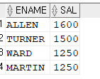
select /*+ gather_plan_statistics */ ename, sal
  from emp
  where job='SALESMAN'
  order by sal desc;
  
----------------------------------------------------------------------------------------------------------------
| Id  | Operation          | Name | Starts | E-Rows | A-Rows |   A-Time   | Buffers |  OMem |  1Mem | Used-Mem |
----------------------------------------------------------------------------------------------------------------
|   0 | SELECT STATEMENT   |      |      1 |        |      4 |00:00:00.01 |       7 |       |       |          |
|   1 |  SORT ORDER BY     |      |      1 |      4 |      4 |00:00:00.01 |       7 |  2048 |  2048 | 2048  (0)|
|*  2 |   TABLE ACCESS FULL| EMP  |      1 |      4 |      4 |00:00:00.01 |       7 |       |       |          |
----------------------------------------------------------------------------------------------------------------

튜닝 후

select /*+ gather_plan_statistics index_desc(emp emp_sal) */ ename, sal
  from emp
  where job = 'SALESMAN' and sal >=0;

SELECT * 
FROM TABLE(dbms_xplan.display_cursor(null,null,'ALLSTATS LAST'));

문제2. 아래의 SQL을 튜닝하기 필요하면 인덱스도 생성!

튜닝 전

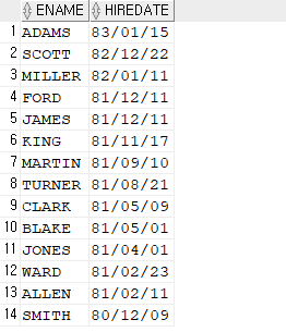
select /*+ gather_plan_statistics */ ename, hiredate
  from emp
  order by hiredate desc;

튜닝 후

-- 인덱스 생성
create index emp_hiredate on emp(hiredate);
-- 튜닝하기
select /*+ gather_plan_statistics index_desc(emp emp_hiredate) */ ename, hiredate
  from emp
  where hiredate < to_date('9999/12/31','RRRR/MM/DD');

➡️ 정렬이 잘 되었음!!

💡참고

인덱스 전체를 스캔하는 조건 : 1. 문자 > '  '
                          2. 숫자 >= 0
                          3. 날짜 < to_date('9999/12/31', 'RRRR/MM/DD')

문제3. 아래의 SQL을 튜닝하기

튜닝 전

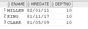
select /*+ gather_plan_statistics */ ename, hiredate, deptno
  from emp
  where deptno=10
  order by hiredate desc;
  
----------------------------------------------------------------------------------------------------------------
| Id  | Operation          | Name | Starts | E-Rows | A-Rows |   A-Time   | Buffers |  OMem |  1Mem | Used-Mem |
----------------------------------------------------------------------------------------------------------------
|   0 | SELECT STATEMENT   |      |      1 |        |      3 |00:00:00.01 |       7 |       |       |          |
|   1 |  SORT ORDER BY     |      |      1 |      3 |      3 |00:00:00.01 |       7 |  2048 |  2048 | 2048  (0)|
|*  2 |   TABLE ACCESS FULL| EMP  |      1 |      3 |      3 |00:00:00.01 |       7 |       |       |          |
----------------------------------------------------------------------------------------------------------------

튜닝 후!

 select /*+ gather_plan_statistics index_desc(emp emp_hiredate) */ ename, hiredate, deptno
  from emp
  where deptno=10
  and hiredate < to_date('9999/12/31','RRRR/MM/DD');

-------------------------------------------------------------------------------------------------------
| Id  | Operation                    | Name         | Starts | E-Rows | A-Rows |   A-Time   | Buffers |
-------------------------------------------------------------------------------------------------------
|   0 | SELECT STATEMENT             |              |      1 |        |      3 |00:00:00.01 |       2 |
|*  1 |  TABLE ACCESS BY INDEX ROWID | EMP          |      1 |      3 |      3 |00:00:00.01 |       2 |
|*  2 |   INDEX RANGE SCAN DESCENDING| EMP_HIREDATE |      1 |     14 |     14 |00:00:00.01 |       1 |
-------------------------------------------------------------------------------------------------------

➡️ and로 연결해주면 된다. 정렬도 잘 되었고 버퍼의 갯수도 줄어들었음!

문제4. 아래의 SQL을 튜닝하기

튜닝 전 : SORT AGGREGATE 가 들어가있다. 바람직하지 않음!!

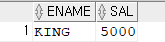
select /*+ gather_plan_statistics */ max(sal)
  from emp;
 
------------------------------------------------------------------------------------------------
| Id  | Operation                  | Name    | Starts | E-Rows | A-Rows |   A-Time   | Buffers |
------------------------------------------------------------------------------------------------
|   0 | SELECT STATEMENT           |         |      1 |        |      1 |00:00:00.01 |       1 |
|   1 |  SORT AGGREGATE            |         |      1 |      1 |      1 |00:00:00.01 |       1 |
|   2 |   INDEX FULL SCAN (MIN/MAX)| EMP_SAL |      1 |      1 |      1 |00:00:00.01 |       1 |
------------------------------------------------------------------------------------------------

➡️ 테이블이나 인덱스를 full scan하고 나서, 최댓값을 보아야 해서 sort가 일어난다.

튜닝 후

select /*+ gather_plan_statistics index_desc(emp emp_sal) */ sal
  from emp
  where sal >= 0 and rownum = 1;

--------------------------------------------------------------------------------------------------
| Id  | Operation                    | Name    | Starts | E-Rows | A-Rows |   A-Time   | Buffers |
--------------------------------------------------------------------------------------------------
|   0 | SELECT STATEMENT             |         |      1 |        |      1 |00:00:00.01 |       1 |
|*  1 |  COUNT STOPKEY               |         |      1 |        |      1 |00:00:00.01 |       1 |
|*  2 |   INDEX RANGE SCAN DESCENDING| EMP_SAL |      1 |     14 |      1 |00:00:00.01 |       1 |
--------------------------------------------------------------------------------------------------

➡️ 인덱스를 descending 하는 상태에서 맨 위에있는 한개를 가져오면 max 값!
❓ COUNT STOPKEY 는 rownum 때문에 나온애다!

문제5. 아래의 SQL을 튜닝하기

튜닝 전 : emp table을 2번이나 읽고있다.

select /*+ gather_plan_statistics */ ename, sal
  from emp
  where sal = ( select max(sal)
                 from emp);

--------------------------------------------------------------------------------------------------
| Id  | Operation                    | Name    | Starts | E-Rows | A-Rows |   A-Time   | Buffers |
--------------------------------------------------------------------------------------------------
|   0 | SELECT STATEMENT             |         |      1 |        |      1 |00:00:00.01 |       3 |
|   1 |  TABLE ACCESS BY INDEX ROWID | EMP     |      1 |      1 |      1 |00:00:00.01 |       3 |
|*  2 |   INDEX RANGE SCAN           | EMP_SAL |      1 |      1 |      1 |00:00:00.01 |       2 |
|   3 |    SORT AGGREGATE            |         |      1 |      1 |      1 |00:00:00.01 |       1 |
|   4 |     INDEX FULL SCAN (MIN/MAX)| EMP_SAL |      1 |      1 |      1 |00:00:00.01 |       1 |
--------------------------------------------------------------------------------------------------

튜닝 후

select /*+ gather_plan_statistics index_desc(emp emp_sal) */ ename, sal
  from emp
  where sal >= 0 and rownum = 1;

---------------------------------------------------------------------------------------------------
| Id  | Operation                     | Name    | Starts | E-Rows | A-Rows |   A-Time   | Buffers |
---------------------------------------------------------------------------------------------------
|   0 | SELECT STATEMENT              |         |      1 |        |      1 |00:00:00.01 |       2 |
|*  1 |  COUNT STOPKEY                |         |      1 |        |      1 |00:00:00.01 |       2 |
|   2 |   TABLE ACCESS BY INDEX ROWID | EMP     |      1 |     14 |      1 |00:00:00.01 |       2 |
|*  3 |    INDEX RANGE SCAN DESCENDING| EMP_SAL |      1 |     14 |      1 |00:00:00.01 |       1 |
---------------------------------------------------------------------------------------------------

➡️ 버퍼의 갯수도 줄어들었다.

문제6. (SQLP에 자주나오는 문제) 아래의 SQL을 튜닝하세요

@demo
create index emp_deptno_sal on emp(deptno,sal);

튜닝 전

select /*+ gather_plan_statistics */ deptno, max(sal)
  from emp
  where deptno = 20
  group by deptno;
  
-------------------------------------------------------------------------------------------------
| Id  | Operation            | Name           | Starts | E-Rows | A-Rows |   A-Time   | Buffers |
-------------------------------------------------------------------------------------------------
|   0 | SELECT STATEMENT     |                |      1 |        |      1 |00:00:00.01 |       1 |
|   1 |  SORT GROUP BY NOSORT|                |      1 |      5 |      1 |00:00:00.01 |       1 |
|*  2 |   INDEX RANGE SCAN   | EMP_DEPTNO_SAL |      1 |      5 |      5 |00:00:00.01 |       1 |
-------------------------------------------------------------------------------------------------

튜닝 후

select /*+ gather_plan_statistics index_desc(emp emp_deptno_sal) */ deptno, sal
  from emp
  where deptno = 20 ;
# 이렇게만 작성하면 deptno가 20번인 애들을 descending하게 가져온다. 
# 그렇다면 여기서 rownum이 1인 애를 가져오면 max값과 같다.

select /*+ gather_plan_statistics index_desc(emp emp_deptno_sal) */ deptno, sal
  from emp
  where deptno = 20 and rownum = 1;

---------------------------------------------------------------------------------------------------------
| Id  | Operation                    | Name           | Starts | E-Rows | A-Rows |   A-Time   | Buffers |
---------------------------------------------------------------------------------------------------------
|   0 | SELECT STATEMENT             |                |      1 |        |      1 |00:00:00.01 |       1 |
|*  1 |  COUNT STOPKEY               |                |      1 |        |      1 |00:00:00.01 |       1 |
|*  2 |   INDEX RANGE SCAN DESCENDING| EMP_DEPTNO_SAL |      1 |      5 |      1 |00:00:00.01 |       1 |
---------------------------------------------------------------------------------------------------------

문제7. 아래의 SQL을 튜닝하는데 필요한 인덱스도 적절히 생성해서 튜닝하기

환경구성

create table sales700 as select * from sh.sales;

튜닝 전

select channel_id, max(amount_sold)
  from sales700
  where channel_id = 3
  group by channel_id;

튜닝 후

-- 인덱스 만들기
create index sales700_indx1 on sales700(channel_id,amount_sold);

-- 튜닝
select /*+ gather_plan_statistics index_desc(s sales700_indx1) */ channel_id, amount_sold
  from sales700 s
  where channel_id = 3 and rownum = 1;

---------------------------------------------------------------------------------------------------------
| Id  | Operation                    | Name           | Starts | E-Rows | A-Rows |   A-Time   | Buffers |
---------------------------------------------------------------------------------------------------------
|   0 | SELECT STATEMENT             |                |      1 |        |      1 |00:00:00.01 |       3 |
|*  1 |  COUNT STOPKEY               |                |      1 |        |      1 |00:00:00.01 |       3 |
|*  2 |   INDEX RANGE SCAN DESCENDING| SALES700_INDX1 |      1 |    598K|      1 |00:00:00.01 |       3 |
---------------------------------------------------------------------------------------------------------

✏️ 보이지 않는 인덱스 만들기

(p.4-38)

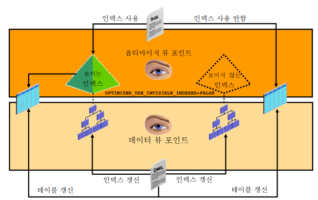
💡 옵티마이저로 하여금 인덱스를 못보게 하는 이유

1. 특정 인덱스를 엑세스 하지 않는 실행계획을 일부러 만들게 하고 싶을 때
예)
대한항공에서 새로운 인덱스를 만들었다가 티켓팅이 안되는 현상 발생
함부로 인덱스를 삭제했는데 그 인덱스가 다른 SQL에서는 중요하게 사용이 된 경우라면 
삭제한 인덱스를 생성해야하는데, 시간이 너무 오래걸리고 UNDO나 TEMP 테이블 스페이스가 full이 
날 수도 있기때문에 함부로 인덱스를 생성해서는 안된다!!
2. 불필요한 인덱스여서 drop을 하고싶다! 그런데 이 인덱스가 어느 SQL에서 사용되는지 파악을 잘 못할때 잠깐 인덱스를 옵티마이저가 안보이게 합니다.

실습

@demo
create index emp_sal on emp(sal);

select /*+ gather_plan_statistics */ ename, sal
  from emp
  where sal = 3000;

-------------------------------------------------------------------------------------------------
| Id  | Operation                   | Name    | Starts | E-Rows | A-Rows |   A-Time   | Buffers |
-------------------------------------------------------------------------------------------------
|   0 | SELECT STATEMENT            |         |      1 |        |      2 |00:00:00.01 |       2 |
|   1 |  TABLE ACCESS BY INDEX ROWID| EMP     |      1 |      2 |      2 |00:00:00.01 |       2 |
|*  2 |   INDEX RANGE SCAN          | EMP_SAL |      1 |      2 |      2 |00:00:00.01 |       1 |
-------------------------------------------------------------------------------------------------

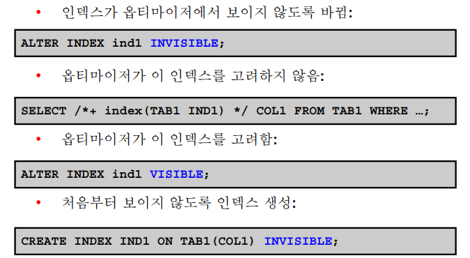
문제1. 책 4-39를 보고 옵티마이저가 emp_sal 인덱스를 못보게 해보기

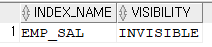
alter index emp_sal invisible;

select /*+ gather_plan_statistics */ ename, sal
  from emp
  where sal = 3000;
 
SELECT * 
FROM TABLE(dbms_xplan.display_cursor(null,null,'ALLSTATS LAST')); 

------------------------------------------------------------------------------------
| Id  | Operation         | Name | Starts | E-Rows | A-Rows |   A-Time   | Buffers |
------------------------------------------------------------------------------------
|   0 | SELECT STATEMENT  |      |      1 |        |      2 |00:00:00.01 |       7 |
|*  1 |  TABLE ACCESS FULL| EMP  |      1 |      2 |      2 |00:00:00.01 |       7 |
------------------------------------------------------------------------------------

➡️ full table scan이라고 나옴!

-- invisible 되었는지 확인
select index_name, visibility 
 from user_indexes
 where table_name='EMP';

⭐ 인덱스를 drop해야하는 상황에서 바로 drop하지 말고 invisible 하고 문제가 없다면 drop하자!

문제2. 그럼 다시 옵티마이저가 emp_sal 인덱스가 보이도록 설정하기

alter index emp_sal visible;

select index_name, visibility 
 from user_indexes
 where table_name='EMP';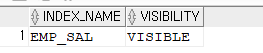

✏️ IOT (Index Organization Table)

💡 IOT란 테이블 랜덤 엑세스가 발생하지 않도록 테이블을 아예 인덱스 구조로 생성한 object이다!
IOT는 인덱스 리프블럭에 모든 데이터를 다 포함시키므로 테이블 랜덤 엑세스를 하지 않아도 된다는 장점이 있다.
(테이블인데 인덱스 테이블이다!!)

실습 IOT table을 생성해보기

create table emp_iot
 (
  EMPNO       NUMBER(4)     primary key , 
  ENAME       VARCHAR2(10)         NULL, 
  JOB         VARCHAR2(9)          NULL, 
  MGR         NUMBER(4)            NULL, 
  HIREDATE    DATE                 NULL, 
  SAL         NUMBER(7, 2)         NULL, 
  COMM        NUMBER(7, 2)         NULL, 
  DEPTNO      NUMBER(2)            NULL  )
organization  index; 

insert  into  emp_iot
        select  *
           from emp;

commit;

➡️ 일반 테이블 생성과 같은데 organization index;를 써야하고 empno에 프라이머리키 제약이 걸려있어야 한다.

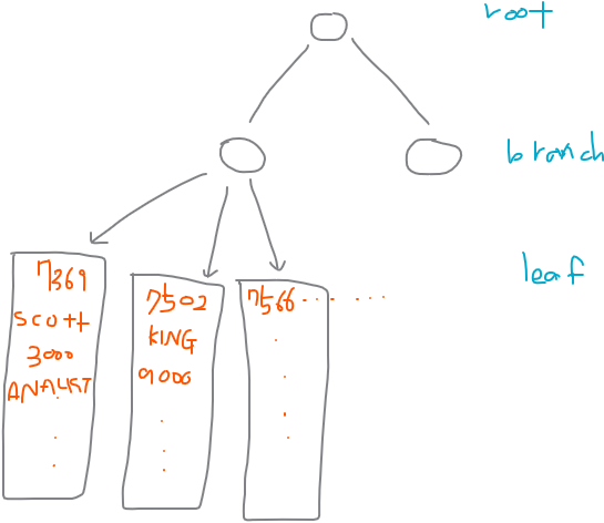
인덱스 안에 empno에 대한 모든 정보가 들어가있다. 7369 사원 이름은 scott, 월급은 3000 등..

💡 자주 조회하는 검색이 중요한 테이블들은 iot로 구성할 것을 권장!

문제1. 사원번호가 7788번인 사원의 모든 컬럼의 데이터를 가져오는 아래의 쿼리 성는ㅇ을 비교해보기

✔️ 튜닝전

select /*+ gather_plan_statistics */ *
  from emp
  where empno=7788;

SELECT * 
FROM TABLE(dbms_xplan.display_cursor(null,null,'ALLSTATS LAST')); 

------------------------------------------------------------------------------------
| Id  | Operation         | Name | Starts | E-Rows | A-Rows |   A-Time   | Buffers |
------------------------------------------------------------------------------------
|   0 | SELECT STATEMENT  |      |      1 |        |      1 |00:00:00.01 |       7 |
|*  1 |  TABLE ACCESS FULL| EMP  |      1 |      1 |      1 |00:00:00.01 |       7 |
------------------------------------------------------------------------------------

✔️ 튜닝후

select /*+ gather_plan_statistics */ *
  from emp_iot
  where empno=7788;

SELECT * 
FROM TABLE(dbms_xplan.display_cursor(null,null,'ALLSTATS LAST')); 

-------------------------------------------------------------------------------------------------
| Id  | Operation         | Name              | Starts | E-Rows | A-Rows |   A-Time   | Buffers |
-------------------------------------------------------------------------------------------------
|   0 | SELECT STATEMENT  |                   |      1 |        |      1 |00:00:00.01 |       1 |
|*  1 |  INDEX UNIQUE SCAN| SYS_IOT_TOP_87720 |      1 |      1 |      1 |00:00:00.01 |       1 |
-------------------------------------------------------------------------------------------------

➡️ 버퍼의 갯수가 7개에서 1개로 줄었다!

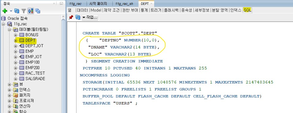
문제2. dept테이블을 가지고 dept_iot테이블을 생성하고 아래의 튜닝전, 튜닝후를 비교하기

create table dept_iot
 (
  DEPTNO       NUMBER(10)     primary key , 
  DNAME       VARCHAR2(14)         NULL, 
  LOC       VARCHAR2(13)         NULL)
organization  index; 

insert  into  dept_iot
        select  *
           from dept;

✔️ 튜닝전

select /*+ gather_plan_statistics */ *
  from dept
  where deptno=10;

SELECT * 
FROM TABLE(dbms_xplan.display_cursor(null,null,'ALLSTATS LAST')); 

------------------------------------------------------------------------------------
| Id  | Operation         | Name | Starts | E-Rows | A-Rows |   A-Time   | Buffers |
------------------------------------------------------------------------------------
|   0 | SELECT STATEMENT  |      |      1 |        |      1 |00:00:00.01 |       7 |
|*  1 |  TABLE ACCESS FULL| DEPT |      1 |      1 |      1 |00:00:00.01 |       7 |
------------------------------------------------------------------------------------

✔️ 튜닝후

select /*+ gather_plan_statistics */ *
  from dept_iot
  where deptno=10;

SELECT * 
FROM TABLE(dbms_xplan.display_cursor(null,null,'ALLSTATS LAST')); 

-------------------------------------------------------------------------------------------------
| Id  | Operation         | Name              | Starts | E-Rows | A-Rows |   A-Time   | Buffers |
-------------------------------------------------------------------------------------------------
|   0 | SELECT STATEMENT  |                   |      1 |        |      1 |00:00:00.01 |       1 |
|*  1 |  INDEX UNIQUE SCAN| SYS_IOT_TOP_87722 |      1 |      1 |      1 |00:00:00.01 |       1 |
-------------------------------------------------------------------------------------------------

💡 sqldeveloper에서 아래 내용 가져와도 됨!

✔️ iot 테이블의 장점과 단점

1. 장점

1) 검색 성능이 좋아진다.
2) 저장 공간이 절약된다.

2. 단점

1) insert 작업시 성능이 떨어진다.

문제3. emp테이블과 emp_iot 테이블의 저장공간을 비교하기

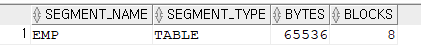
✅ emp 테이블

select segment_name, segment_type, bytes, blocks
  from user_segments
  where segment_name='EMP';

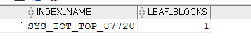
✅ emp_iot 테이블

analyze table emp_iot compute statistics; -- 분석 해주어야 함!!

select index_name, leaf_blocks
  from user_indexes
  where table_name='EMP_IOT';

➡️ emp_iot의 경우는 블락이 1개이다.

✏️ 클러스터 테이블

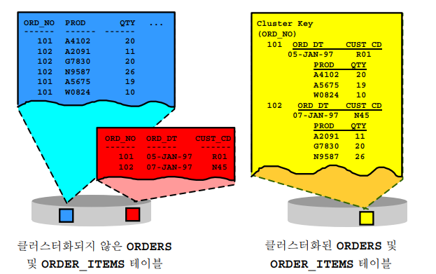
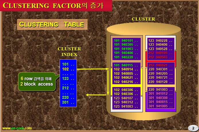
💡 클러스터 테이블이란 클러스터 키 값이 같은 레코드가 한 블럭에 모이도록 저장하는 구조의 테이블을 말한다!

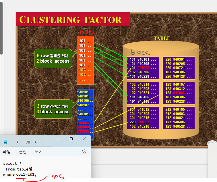
✔️ 클러스터링 팩터의 의미 이해

💡 인덱스의 클러스터링 팩터(clustering factor)란 인덱스를 통해 엑세스 되는 데이터가 얼마나 같은 블럭 안에 모여있느냐라는 것인데, 클러스터링 팩터가 좋다는 것은 엑세스 되는 데이터가 같은 블럭 안에 잘 모여있다는 것이다. 아래 화면 보면 위에가 더 좋다! 같은 블럭안에 데이터가 더 많으니까.

✔️ clustering factor 테스트

-- 예쁘게 정렬된 데이터가 있음
create table  emp5000
pctfree 0
as
  select t2.*, lpad('x', 630) x 
    from dba_objects t2
    order by object_id;

-- 랜덤으로 흩어져있음
create table emp6000
pctfree 0
as
  select t2.*, lpad('x', 630) x 
    from dba_objects t2
    order by dbms_random.value;

create  index   emp5000_object_id  on  emp5000(object_id);
create  index   emp6000_object_id  on  emp6000(object_id);

✅ 위의 인덱스의 클러스터링 팩터를 조사한다.

analyze table emp5000 compute statistics;
analyze table emp6000 compute statistics;

select   i.index_name, t.blocks, i.clustering_factor,  t.num_rows
  from   user_indexes  i,  user_tables   t
 where   i.table_name = t.table_name
   and   t.table_name in ('EMP5000','EMP6000');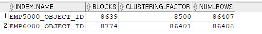

➡️ 클러스터링 팩터가 작을 수록 좋은 인덱스이다.

문제1. 아래 2개의 SQL의 퍼버의 갯수 확인하기

select /*+ gather_plan_statistics */ * 
  from emp5000
  where object_id between 1 and 300;
 
SELECT * 
FROM TABLE(dbms_xplan.display_cursor(null,null,'ALLSTATS LAST')); 

--------------------------------------------------------------------------------------------------------------------
| Id  | Operation                   | Name              | Starts | E-Rows | A-Rows |   A-Time   | Buffers | Reads  |
--------------------------------------------------------------------------------------------------------------------
|   0 | SELECT STATEMENT            |                   |      1 |        |     50 |00:00:00.05 |       7 |      1 |
|   1 |  TABLE ACCESS BY INDEX ROWID| EMP5000           |      1 |    295 |     50 |00:00:00.05 |       7 |      1 |
|*  2 |   INDEX RANGE SCAN          | EMP5000_OBJECT_ID |      1 |    295 |     50 |00:00:00.04 |       2 |      1 |
--------------------------------------------------------------------------------------------------------------------
  
select /*+ gather_plan_statistics */ * 
  from emp6000
  where object_id between 1 and 300;

SELECT * 
FROM TABLE(dbms_xplan.display_cursor(null,null,'ALLSTATS LAST')); 

--------------------------------------------------------------------------------------------------------------------
| Id  | Operation                   | Name              | Starts | E-Rows | A-Rows |   A-Time   | Buffers | Reads  |
--------------------------------------------------------------------------------------------------------------------
|   0 | SELECT STATEMENT            |                   |      1 |        |     50 |00:00:00.04 |      52 |      1 |
|   1 |  TABLE ACCESS BY INDEX ROWID| EMP6000           |      1 |    295 |     50 |00:00:00.04 |      52 |      1 |
|*  2 |   INDEX RANGE SCAN          | EMP6000_OBJECT_ID |      1 |    295 |     50 |00:00:00.04 |       2 |      1 |
--------------------------------------------------------------------------------------------------------------------

➡️ 테이블을 만들 때 order by를 하면 좋은 클러스터를 가질 수 있지만 일부러 이렇게 하지는 않는다. 위 예제는 인덱스의 클러스터링 팩터의 예제이다.

💡 다음은 테이블을 생성할 때 클러스터링 팩터가 좋은 클러스터 테이블을 생성하는 방법!

✔️ 클러스터 테이블의 종류 2가지

1. 인덱스 클러스터 테이블
* 단일 테이블 인덱스 클러스터
* 다중 테이블 인덱스 클러스터
✅ 단일 테이블 인덱스 클러스터

✅ 다중 테이블 인덱스 클러스터

2. 해쉬 클러스터 테이블

✔️ 다중 테이블 인덱스 클러스터 생성 실습

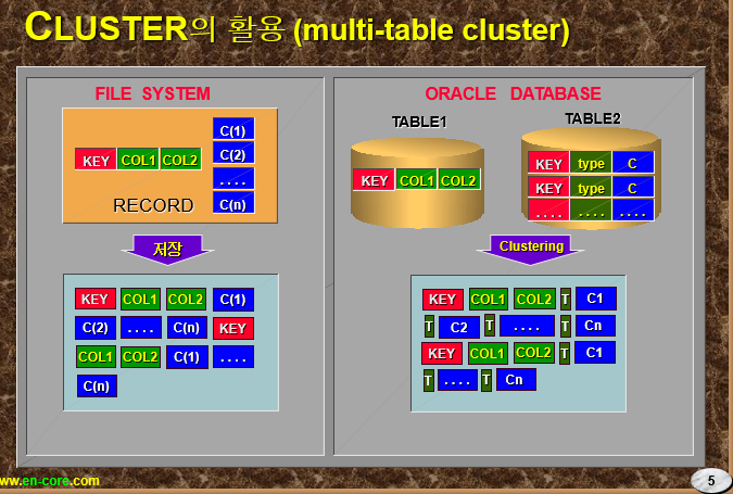
💡 다중 테이블 인덱스 클러스터는 여러 테이블들의 레코드를 하나의 물리적 공간에 같이 저장해두는 방식 여러 테이블들을 서로 조인된 상태로 저장해둔다

➡️ emp 와 dept 를 가지고 다중 클러스터 테이블 구현

1. 클러스터를 생성한다.

alter   table  emp   modify  deptno  number(10);
alter   table  dept  modify  deptno  number(10); 

create  cluster  c_deptno
( deptno    number(10)  )  index;

2. 클러스터 인덱스를 생성한다.

create  index   i_deptno   on   cluster  c_deptno ;

3. 클러스터 테이블을 생성한다.

create  table  emp_cluster  
cluster   c_deptno(deptno)
as
 select  * from  emp; 

create  table dept_cluster
cluster  c_deptno(deptno)
as
 select  * from  dept ;

4. 조회해보기

select* from emp_cluster;
select* from dept_cluster;

문제1. 아래의 SQL 문의 성능을 보고 비교하기

✔️ 튜닝 전

select /*+ gather_plan_statistics use_nl(e d) */ e.ename, d.loc, e.sal, e.hiredate, d.dname, e.deptno, e.mgr
  from emp e, dept d
  where e.deptno = d.deptno and d.loc='DALLAS';

-------------------------------------------------------------------------------------
| Id  | Operation          | Name | Starts | E-Rows | A-Rows |   A-Time   | Buffers |
-------------------------------------------------------------------------------------
|   0 | SELECT STATEMENT   |      |      1 |        |      5 |00:00:00.01 |      14 |
|   1 |  NESTED LOOPS      |      |      1 |      5 |      5 |00:00:00.01 |      14 |
|*  2 |   TABLE ACCESS FULL| DEPT |      1 |      1 |      1 |00:00:00.01 |       7 |
|*  3 |   TABLE ACCESS FULL| EMP  |      1 |      5 |      5 |00:00:00.01 |       7 |
-------------------------------------------------------------------------------------

✔️ 튜닝 후

select /*+ gather_plan_statistics use_nl(e d) */ e.ename, d.loc, e.sal, e.hiredate, d.dname, e.deptno, e.mgr
  from emp_cluster e, dept_cluster d
  where e.deptno = d.deptno and d.loc='DALLAS';

------------------------------------------------------------------------------------------------
| Id  | Operation             | Name         | Starts | E-Rows | A-Rows |   A-Time   | Buffers |
------------------------------------------------------------------------------------------------
|   0 | SELECT STATEMENT      |              |      1 |        |      5 |00:00:00.01 |       9 |
|   1 |  NESTED LOOPS         |              |      1 |      5 |      5 |00:00:00.01 |       9 |
|*  2 |   TABLE ACCESS FULL   | DEPT_CLUSTER |      1 |      1 |      1 |00:00:00.01 |       7 |
|*  3 |   TABLE ACCESS CLUSTER| EMP_CLUSTER  |      1 |      5 |      5 |00:00:00.01 |       2 |
------------------------------------------------------------------------------------------------

문제2. emp_cluster와 dept_cluster가 물리적으로 정말 같은 공간에 존재하는지 확인하기

select   d.deptno, e.empno,  e.ename, d.loc,
         dbms_rowid.rowid_block_number(d.rowid)  deptno_block_no,
            dbms_rowid.rowid_block_number(e.rowid)  emp_block_no
   from    dept_cluster    d,  emp_cluster   e
   where   e.deptno = d.deptno
   order by    d.deptno ;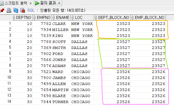

문제3. 아래의 테이블을 스캇유저에서 생성하고, 아래의 SQL을 튜닝하는데 클러스터 테이블로 생성해서 튜닝하기

create table sales
as
  select * from sh.sales;
 
create table products
as
  select * from sh.products;

1. 클러스터를 생성한다.

-- 연결고리 컬럼을 데이터타입이 같게 만들기
alter   table  sales   modify  PROD_ID  NUMBER;
alter   table  products  modify  PROD_ID  NUMBER; 

-- 클러스터 만들기
create  cluster  c_prod_id
( PROD_ID  NUMBER(38)  )  index;

2. 클러스터 인덱스를 생성한다.

create  index   i_prod_id  on   cluster  c_prod_id ;

3. 클러스터 테이블을 생성한다.

-- 클러스터 넣어서 테이블 생성
create  table  sales_cluster  
cluster   c_prod_id(prod_id)
as
 select  * from  sales; 

create  table products_cluster
cluster  c_prod_id(prod_id)
as
 select  * from  products ;

✔️ 튜닝 전

SELECT  /*+ gather_plan_statistics leading(p s) use_nl(s) */ p.prod_name, sum(s.amount_sold)
        from sales   s,  products  p 
        where  s.prod_id = p.prod_id
         and   p.prod_id = 40
        group by p.prod_name;  

SELECT * 
FROM TABLE(dbms_xplan.display_cursor(null,null,'ALLSTATS LAST')); 

---------------------------------------------------------------------------------------------------------------------
| Id  | Operation           | Name     | Starts | E-Rows | A-Rows |   A-Time   | Buffers |  OMem |  1Mem | Used-Mem |
---------------------------------------------------------------------------------------------------------------------
|   0 | SELECT STATEMENT    |          |      1 |        |      1 |00:00:00.01 |    4444 |       |       |          |
|   1 |  HASH GROUP BY      |          |      1 |  46982 |      1 |00:00:00.01 |    4444 |  3403K|  1297K|  816K (0)|
|   2 |   NESTED LOOPS      |          |      1 |  46982 |  27114 |00:00:00.03 |    4444 |       |       |          |
|*  3 |    TABLE ACCESS FULL| PRODUCTS |      1 |      1 |      1 |00:00:00.01 |       4 |       |       |          |
|*  4 |    TABLE ACCESS FULL| SALES    |      1 |  46982 |  27114 |00:00:00.02 |    4440 |       |       |          |
---------------------------------------------------------------------------------------------------------------------

✔️ 튜닝 후

SELECT  /*+ gather_plan_statistics leading(p s) use_nl(s) */ p.prod_name, sum(s.amount_sold)
        from sales_cluster  s,  products_cluster  p 
        where  s.prod_id = p.prod_id
         and   p.prod_id = 40
        group by p.prod_name;  

SELECT * 
FROM TABLE(dbms_xplan.display_cursor(null,null,'ALLSTATS LAST')); 

--------------------------------------------------------------------------------------------------------------------------------
| Id  | Operation              | Name             | Starts | E-Rows | A-Rows |   A-Time   | Buffers |  OMem |  1Mem | Used-Mem |
--------------------------------------------------------------------------------------------------------------------------------
|   0 | SELECT STATEMENT       |                  |      1 |        |      1 |00:00:00.01 |     244 |       |       |          |
|   1 |  HASH GROUP BY         |                  |      1 |  30803 |      1 |00:00:00.01 |     244 |  3322K|  1297K|  797K (0)|
|   2 |   NESTED LOOPS         |                  |      1 |  30803 |  27114 |00:00:00.01 |     244 |       |       |          |
|   3 |    TABLE ACCESS CLUSTER| PRODUCTS_CLUSTER |      1 |      1 |      1 |00:00:00.01 |     122 |       |       |          |
|*  4 |     INDEX UNIQUE SCAN  | I_PROD_ID        |      1 |      1 |      1 |00:00:00.01 |       1 |       |       |          |
|*  5 |    TABLE ACCESS CLUSTER| SALES_CLUSTER    |      1 |  30407 |  27114 |00:00:00.01 |     122 |       |       |          |
--------------------------------------------------------------------------------------------------------------------------------

➡️ 아무리 SQL을 튜닝해도 성능 개선이 안보이면 저장 구조를 IOT나 클러스터 테이블로 구성하는것을 고려해보아야 한다.
➡️ 버퍼의 갯수가 4444개 -> 244개 !

✏️ 해쉬 클러스터 테이블 생성

해쉬 클러스터 생성

create cluster username_cluster# ( username varchar2(30) ) 
hashkeys 100 size 50;

클러스터 테이블 생성

create table user_cluster
cluster username_cluster# ( username )
as
select * from all_users;

일반 테이블을 생성( 일반 테이블과 해쉬 테이블의 성능을 비교하려고)

create table user_regular as select * from all_users;

create unique index user_regular_idx on user_regular(username);

alter table user_regular modify user_id null;
alter table user_cluster modify user_id null;

일반 테이블과 해쉬 클러스터 테이블의 성능 비교 테스트 PL/SQL

@t.sql

declare
  l_user_id user_regular.user_id%type;
begin
  for c in (select owner from all_objects where owner <> 'PUBLIC')
  loop
    select user_id into l_user_id from user_regular where username = c.owner;
    select user_id into l_user_id from user_cluster where username = c.owner;
  end loop;
end;
/

@tf.sql
@trace_file.sql

TRACE_FILE_NAME
--------------------------------------------------------------------------------
/u01/app/oracle/diag/rdbms/racdb/racdb1/trace/racdb1_ora_1749.trc

@tk

💡 위 실습하면서 필요한 sql 스크립트들! SQL trace를 뜨는 스크립트들임
t.sql, tk.sql, tf.sql, trace_file.sql

SCOTT @ racdb1 > @t.sql
Session altered.
SCOTT @ racdb1 > l --l하면 방금 수행한 sql을 볼 수 있다.
  1* alter session set events '10046 trace name context forever, level 12'

⭐ IOT, 클러스터 테이블을 배웠는데 이 테이블을 테이블 구조 자체가 일반 테이블과는 다른 구조이다. IOT는 인덱스에 테이블의 내용을 다 합쳐놓은 테이블이고 클러스터 테이블을 clustering factor가 좋도록 데이터를 물리적으로 재구성한 테이블이다. 검색하려는 데이터를 같은 블럭 안에 몰아넣은 테이블이다.

오늘의 마지막 문제 아래의 SQL을 튜닝하기

@demo

-- 튜닝전
select /*+ gather_plan_statistics*/ job, max(sal)
  from emp
  where job='SALESMAN'
  group by job;
  
---------------------------------------------------------------------------------------
| Id  | Operation            | Name | Starts | E-Rows | A-Rows |   A-Time   | Buffers |
---------------------------------------------------------------------------------------
|   0 | SELECT STATEMENT     |      |      1 |        |      1 |00:00:00.01 |       7 |
|   1 |  SORT GROUP BY NOSORT|      |      1 |      4 |      1 |00:00:00.01 |       7 |
|*  2 |   TABLE ACCESS FULL  | EMP  |      1 |      4 |      4 |00:00:00.01 |       7 |
---------------------------------------------------------------------------------------

✔️ 튜닝 후!

-- 인덱스 만들기
create index emp_indx1 on emp(job,sal);

-- 튜닝
select /*+ gather_plan_statistics index_desc(emp emp_indx1) */ job, sal
  from emp 
  where job='SALESMAN' and rownum = 1;

SELECT * 
FROM TABLE(dbms_xplan.display_cursor(null,null,'ALLSTATS LAST'));

----------------------------------------------------------------------------------------------------
| Id  | Operation                    | Name      | Starts | E-Rows | A-Rows |   A-Time   | Buffers |
----------------------------------------------------------------------------------------------------
|   0 | SELECT STATEMENT             |           |      1 |        |      1 |00:00:00.01 |       1 |
|*  1 |  COUNT STOPKEY               |           |      1 |        |      1 |00:00:00.01 |       1 |
|*  2 |   INDEX RANGE SCAN DESCENDING| EMP_INDX1 |      1 |      4 |      1 |00:00:00.01 |       1 |
----------------------------------------------------------------------------------------------------

망구씨

Slow and steady wins the race.

이전 포스트

[SQL튜닝]23.11.17

다음 포스트

[SQL튜닝]23.11.20

SQL 튜닝

복습! SQL튜닝

✔️ index join scan 방법

💡 인덱스 조인보다 결합 컬럼 인덱스가 훨씬 더 튜닝 SQL이다!

✍🏻 인덱스 관련한 추가 튜닝 내용 1 (결합 컬럼 인덱스의 컬럼 구성 순서의 중요성)

⭐ 튜닝 tip !

✍🏻 인덱스 관련한 추가 튜닝 내용 2 (결합 컬럼 인덱스의 컬럼 구성 순서의 중요성2)

✍🏻 인덱스 관련한 추가 튜닝 내용3 (인덱스를 descending 하게 스캔하기)

✏️ 보이지 않는 인덱스 만들기

⭐ 인덱스를 drop해야하는 상황에서 바로 drop하지 말고 invisible 하고 문제가 없다면 drop하자!

✏️ IOT (Index Organization Table)

✔️ iot 테이블의 장점과 단점

✏️ 클러스터 테이블

✔️ 클러스터링 팩터의 의미 이해

✔️ clustering factor 테스트

✔️ 다중 테이블 인덱스 클러스터 생성 실습

✏️ 해쉬 클러스터 테이블 생성

[SQL튜닝]23.11.17

[SQL튜닝]23.11.21

0개의 댓글