
SQL 튜닝
📖 소목차
1. nested loop 조인
2. hash 조인
3. sort merge 조인
4. 조인 순서의 중요성
5. outer 조인
6. 스칼라 서브쿼리를 이용한 조인 튜닝
7. 조인을 내포한 DML 문 튜닝
8. 고급 조인 테크닉
✏️ 조인 튜닝
❓ 조인 문장을 튜닝할 때 중요한 점 두가지
1. 조인 순서
* ordered : from 절에서 기술한 테이블 순서대로 조인해라
* leading : leading 절 힌트 안에 쓴 테이블 순서대로 조인해라
2. 조인 방법
* nested loop join
* hash join
* sort merge join
✔️ nested loop join (use_nl)
💡 순차적 반복 조인 방법. 두개의 테이블의 데이터를 조인하는데 조인 되는 키컬럼의 데이터를 연결고리 삼아 하나씩 순차적으로 조인하는 조인방법. 조인하려는 data 의 양이 작을 때 유리한 조인 방법
✍🏻 JOIN 흐름!
- 조인 문법과 조인 방법은 서로 다른것이다!
- 조인을 하는 이유는 내가 원하는 데이터가 서로 다른 테이블에 각각 있으면 그 컬럼들을 하나의 결과로 보아야 하기 때문에 조인이 필요하다.
- 조인 문법
1) 오라클 조인 문법
   - equi join
   - non equi join
   - outer join
   - self join
2) 1999 ansi 조인 문법
   - on절을 사용한 조인
   - using 절을 사용한 조인
   - left/right/full outer 조인
   - natural 조인
   - cross 조인
- 조인 방법 : 조인 되는 SQL의 성능을 높이기 위해 알아야한다.
1) nested loop join
2) hash join
3) sort merge join
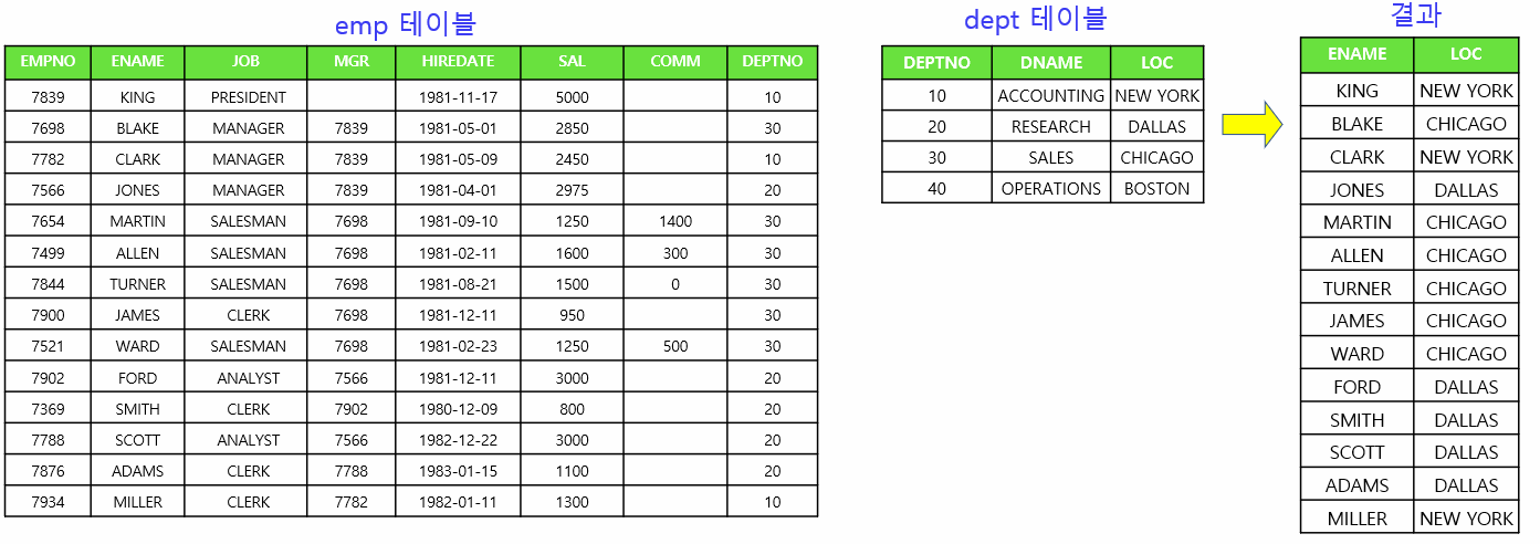
문제1. 사원이름, 월급, 부서위치 출력
select /*+ gather_plan_statistics*/ e.ename, e.sal, d.loc
  from emp e, dept d
  where e.deptno = d.deptno;

SELECT *
FROM TABLE(dbms_xplan.display_cursor(null,null,'ALLSTATS LAST'));

----------------------------------------------------------------------------------------------------------------
| Id  | Operation          | Name | Starts | E-Rows | A-Rows |   A-Time   | Buffers |  OMem |  1Mem | Used-Mem |
----------------------------------------------------------------------------------------------------------------
|   0 | SELECT STATEMENT   |      |      1 |        |     14 |00:00:00.01 |      14 |       |       |          |
|*  1 |  HASH JOIN         |      |      1 |     14 |     14 |00:00:00.01 |      14 |  1696K|  1696K|  987K (0)|
|   2 |   TABLE ACCESS FULL| DEPT |      1 |      4 |      4 |00:00:00.01 |       7 |       |       |          |
|   3 |   TABLE ACCESS FULL| EMP  |      1 |     14 |     14 |00:00:00.01 |       7 |       |       |          |
----------------------------------------------------------------------------------------------------------------
➡️ 지금 출력되는 실행계획은 아래와 같다. 왜 hash join이냐면 full table scan을 했기 때문이다.
1. 조인순서 : DEPT -> EMP
2. 조인방법 : HASH JOIN
❓hash join이 아닌 nested loop join 으로 튜닝해보자
1. 조인 순서를 이용해서 실행계획 출력
문제2. 조인 순서를 일부러 emp->dept 순으로 엑세스 하도록 힌트를 주기
💡(참고) 조인 순서
* ordered : from 절에서 기술한 테이블 순서대로 조인해라
* leading : leading 절 힌트 안에 쓴 테이블 순서대로 조인해라
select /*+ gather_plan_statistics ordered */ e.ename, e.sal, d.loc from emp e, dept d where e.deptno = d.deptno; SELECT * FROM TABLE(dbms_xplan.display_cursor(null,null,'ALLSTATS LAST')); ---------------------------------------------------------------------------------------------------------------- | Id | Operation | Name | Starts | E-Rows | A-Rows | A-Time | Buffers | OMem | 1Mem | Used-Mem | ---------------------------------------------------------------------------------------------------------------- | 0 | SELECT STATEMENT | | 1 | | 14 |00:00:00.01 | 14 | | | | |* 1 | HASH JOIN | | 1 | 14 | 14 |00:00:00.01 | 14 | 1557K| 1557K| 668K (0)| | 2 | TABLE ACCESS FULL| EMP | 1 | 14 | 14 |00:00:00.01 | 7 | | | | | 3 | TABLE ACCESS FULL| DEPT | 1 | 4 | 4 |00:00:00.01 | 7 | | | | ----------------------------------------------------------------------------------------------------------------➡️ EMP를 먼저 읽었다!
문제3. 그렇다면 이번에는 dept->emp순으로 조인되게 하기
: from절의 테이블 순서를 dept 테이블을 먼저 적었음
select /*+ gather_plan_statistics ordered */ e.ename, e.sal, d.loc
  from dept d, emp e
  where e.deptno = d.deptno;

----------------------------------------------------------------------------------------------------------------
| Id  | Operation          | Name | Starts | E-Rows | A-Rows |   A-Time   | Buffers |  OMem |  1Mem | Used-Mem |
----------------------------------------------------------------------------------------------------------------
|   0 | SELECT STATEMENT   |      |      1 |        |     14 |00:00:00.01 |      14 |       |       |          |
|*  1 |  HASH JOIN         |      |      1 |     14 |     14 |00:00:00.01 |      14 |  1696K|  1696K|  985K (0)|
|   2 |   TABLE ACCESS FULL| DEPT |      1 |      4 |      4 |00:00:00.01 |       7 |       |       |          |
|   3 |   TABLE ACCESS FULL| EMP  |      1 |     14 |     14 |00:00:00.01 |       7 |       |       |          |
----------------------------------------------------------------------------------------------------------------
문제4. 이번에는 leading 힌트를 사용해서 조인 순서가 emp->dept 순이 되게 하기
select /*+ gather_plan_statistics leading(e d) */ e.ename, e.sal, d.loc
  from dept d, emp e
  where e.deptno = d.deptno;

SELECT *
FROM TABLE(dbms_xplan.display_cursor(null,null,'ALLSTATS LAST'));

----------------------------------------------------------------------------------------------------------------
| Id  | Operation          | Name | Starts | E-Rows | A-Rows |   A-Time   | Buffers |  OMem |  1Mem | Used-Mem |
----------------------------------------------------------------------------------------------------------------
|   0 | SELECT STATEMENT   |      |      1 |        |     14 |00:00:00.01 |      14 |       |       |          |
|*  1 |  HASH JOIN         |      |      1 |     14 |     14 |00:00:00.01 |      14 |  1557K|  1557K|  644K (0)|
|   2 |   TABLE ACCESS FULL| EMP  |      1 |     14 |     14 |00:00:00.01 |       7 |       |       |          |
|   3 |   TABLE ACCESS FULL| DEPT |      1 |      4 |      4 |00:00:00.01 |       7 |       |       |          |
----------------------------------------------------------------------------------------------------------------
➡️ from절의 순서와 상관없이 emp테이블을 먼저 읽었다!
문제5. leading 힌트를 사용해서 dept->emp 순으로 실행계획이 출력되게 하기
select /*+ gather_plan_statistics leading(d e) */ e.ename, e.sal, d.loc
  from dept d, emp e
  where e.deptno = d.deptno;

SELECT *
FROM TABLE(dbms_xplan.display_cursor(null,null,'ALLSTATS LAST'));

----------------------------------------------------------------------------------------------------------------
| Id  | Operation          | Name | Starts | E-Rows | A-Rows |   A-Time   | Buffers |  OMem |  1Mem | Used-Mem |
----------------------------------------------------------------------------------------------------------------
|   0 | SELECT STATEMENT   |      |      1 |        |     14 |00:00:00.01 |      14 |       |       |          |
|*  1 |  HASH JOIN         |      |      1 |     14 |     14 |00:00:00.01 |      14 |  1696K|  1696K|  987K (0)|
|   2 |   TABLE ACCESS FULL| DEPT |      1 |      4 |      4 |00:00:00.01 |       7 |       |       |          |
|   3 |   TABLE ACCESS FULL| EMP  |      1 |     14 |     14 |00:00:00.01 |       7 |       |       |          |
----------------------------------------------------------------------------------------------------------------
2. use_nl(e) 힌트 사용
문제6. 위의 SQL조인 방법이 nested 조인 방법이 되게 하시오!
select /*+ gather_plan_statistics leading(d e) use_nl(e) */ e.ename, e.sal, d.loc
  from dept d, emp e
  where e.deptno = d.deptno;

-------------------------------------------------------------------------------------
| Id  | Operation          | Name | Starts | E-Rows | A-Rows |   A-Time   | Buffers |
-------------------------------------------------------------------------------------
|   0 | SELECT STATEMENT   |      |      1 |        |     14 |00:00:00.01 |      35 |
|   1 |  NESTED LOOPS      |      |      1 |     14 |     14 |00:00:00.01 |      35 |
|   2 |   TABLE ACCESS FULL| DEPT |      1 |      4 |      4 |00:00:00.01 |       7 |
|*  3 |   TABLE ACCESS FULL| EMP  |      4 |      4 |     14 |00:00:00.01 |      28 |
-------------------------------------------------------------------------------------
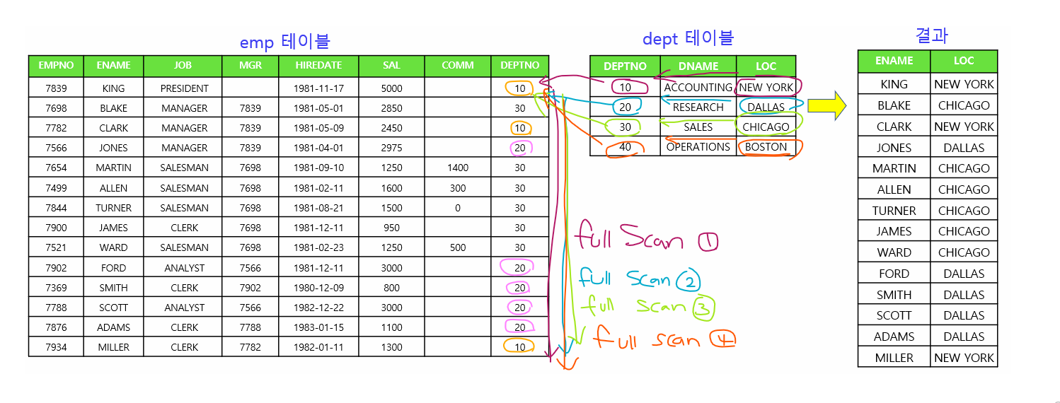
3. nested loop 조인 원리 설명
select /*+ gather_plan_statistics leading(e d) use_nl(d) */ e.ename, d.loc
  from dept d, emp e
  where e.deptno = d.deptno;
💡 우리가 출력하고자 하는것이 이름과 위치라면, 조인순서는 emp->dept leading(e d) / 조인 방법은 nested loop
emp 테이블에서 이름과 deptno를 읽고 dept에 가서 위치를 찾는다. 하나씩 순차적으로 조인!! 반복하고있다. emp테이블을 먼저 읽었으니 14번 조인을 시도한 것이다.
❓ dept -> emp순 으로 조인한다면 몇번 조인시도를 하면 될까?
💡 4번만 조인을 시도한다. 버퍼의 갯수도 차이가 난다!!
# 1. emp -> dept 순일 때 버퍼의 갯수는 105개
-------------------------------------------------------------------------------------
| Id  | Operation          | Name | Starts | E-Rows | A-Rows |   A-Time   | Buffers |
-------------------------------------------------------------------------------------
|   0 | SELECT STATEMENT   |      |      1 |        |     14 |00:00:00.01 |     105 |
|   1 |  NESTED LOOPS      |      |      1 |     14 |     14 |00:00:00.01 |     105 |
|   2 |   TABLE ACCESS FULL| EMP  |      1 |     14 |     14 |00:00:00.01 |       7 |
|*  3 |   TABLE ACCESS FULL| DEPT |     14 |      1 |     14 |00:00:00.01 |      98 |
-------------------------------------------------------------------------------------

# 2. dept -> emp 순일 때 버퍼의 갯수는 35개
-------------------------------------------------------------------------------------
| Id  | Operation          | Name | Starts | E-Rows | A-Rows |   A-Time   | Buffers |
-------------------------------------------------------------------------------------
|   0 | SELECT STATEMENT   |      |      1 |        |     14 |00:00:00.01 |      35 |
|   1 |  NESTED LOOPS      |      |      1 |     14 |     14 |00:00:00.01 |      35 |
|   2 |   TABLE ACCESS FULL| DEPT |      1 |      4 |      4 |00:00:00.01 |       7 |
|*  3 |   TABLE ACCESS FULL| EMP  |      4 |      4 |     14 |00:00:00.01 |      28 |
-------------------------------------------------------------------------------------
문제7. emp, salgrade를 nested loop조인해서 이름, 월급, 등급(grade)를 출력하는데 가장 좋은 조인 순서로 실행계획이 출력되도록 하기
select /*+ gather_plan_statistics leading(s e) use_nl(e) */ e.ename, e.sal, s.grade
 from emp e, salgrade s
 where e.sal between s.losal and s.hisal ;

-----------------------------------------------------------------------------------------
| Id  | Operation          | Name     | Starts | E-Rows | A-Rows |   A-Time   | Buffers |
-----------------------------------------------------------------------------------------
|   0 | SELECT STATEMENT   |          |      1 |        |     14 |00:00:00.01 |      42 |
|   1 |  NESTED LOOPS      |          |      1 |      1 |     14 |00:00:00.01 |      42 |
|   2 |   TABLE ACCESS FULL| SALGRADE |      1 |      5 |      5 |00:00:00.01 |       7 |
|*  3 |   TABLE ACCESS FULL| EMP      |      5 |      1 |     14 |00:00:00.01 |      35 |
-----------------------------------------------------------------------------------------
➡️
leading로 조인 순서를 결정하고use_nl로 조인 방법을 결정하기. 순서가 바뀌어도 상관없지만 이 순서로 하면 헷갈리지 않는다.leading(s e)뒤쪽에 e를 썼다면use_nl(e)도 e로 맞추기!
문제8. 아래의 SQL의 조인 순서를 결정하세요 (방법은 nesed loop)
✔️ 튜닝전
select /*+ ( ? ) */ e.ename, e.sal, d.loc
  from emp e, dept d
  where e.deptno=d.deptno
  and e.ename='KING';
✔️ 튜닝후
: emp는 14건이고 dept는 4건이지만 where절 조건이(KING) 1건이므로 emp 테이블을 먼저 엑세스 하는것이 좋다.select /*+ gather_plan_statistics leading(e d) use_nl(d) */ e.ename, e.sal, d.loc from emp e, dept d where e.deptno=d.deptno and e.ename='KING'; SELECT * FROM TABLE(dbms_xplan.display_cursor(null,null,'ALLSTATS LAST')); ------------------------------------------------------------------------------------- | Id | Operation | Name | Starts | E-Rows | A-Rows | A-Time | Buffers | ------------------------------------------------------------------------------------- | 0 | SELECT STATEMENT | | 1 | | 1 |00:00:00.01 | 14 | | 1 | NESTED LOOPS | | 1 | 1 | 1 |00:00:00.01 | 14 | |* 2 | TABLE ACCESS FULL| EMP | 1 | 1 | 1 |00:00:00.01 | 7 | |* 3 | TABLE ACCESS FULL| DEPT | 1 | 1 | 1 |00:00:00.01 | 7 | -------------------------------------------------------------------------------------➡️
emp -> dept: KING에 대한 부서 위치만 알아내면 되므로 1번만 조인을 시도한다.
dept -> emp: 4번 조인시도를 해서 모두 조인한 다음 KING에 대한 데이터를 따로 검색해서 출력한다.
💡 무조건 테이블의 크기로 leading절의 선행 테이블을 결정하는것이 아니라 where절 조건절에 들어가는 조건 건수를 일일이 확인하고, 조건의 건수가 작은 건수의 테이블이 driving 테이블이 되도록 조인 순서를 정해야한다.
⭐(용어 설명) 조인 순서 : emp -> dept 일 때 emp table은 드라이빙 테이블 혹은 선행 테이블 이라 불린다. dept table은 드라이븐(drived)테이블 혹은 후행 테이블이라 불린다!!
문제9. 아래의 SQL 조인 순서를 결정하기 (조인 방법은 nested loop)
✔️ 튜닝전
select e.ename, e.sal, d.loc
  from emp e, dept d
  where e.deptno = d.deptno
  and e.job='SALESMAN'
  and d.loc='CHICAGO';
✔️ 튜닝후
-- 조건의 건수 구하기
select count(*)
 from emp
 where job = 'SALESMAN'; --4건

select count(*)
 from dept
 where loc='CHICAGO'; --1건

-- 튜닝 (dept의 조건이 1건이므로 dept테이블을 먼저 읽도록)
select /*+ gather_plan_statistics leading(d e) use_nl(e) */ e.ename, e.sal, d.loc
  from emp e, dept d -- emp14건, dept4건
  where e.deptno = d.deptno
  and e.job='SALESMAN'
  and d.loc='CHICAGO';

SELECT *
FROM TABLE(dbms_xplan.display_cursor(null,null,'ALLSTATS LAST'));

-------------------------------------------------------------------------------------
| Id  | Operation          | Name | Starts | E-Rows | A-Rows |   A-Time   | Buffers |
-------------------------------------------------------------------------------------
|   0 | SELECT STATEMENT   |      |      1 |        |      4 |00:00:00.01 |      14 |
|   1 |  NESTED LOOPS      |      |      1 |      1 |      4 |00:00:00.01 |      14 |
|*  2 |   TABLE ACCESS FULL| DEPT |      1 |      1 |      1 |00:00:00.01 |       7 |
|*  3 |   TABLE ACCESS FULL| EMP  |      1 |      1 |      4 |00:00:00.01 |       7 |
-------------------------------------------------------------------------------------
문제10. 아래의 환경을 구성하고 아래 SQL을 튜닝해서 버퍼의 갯수를 비교하기
create  table  sales200
 as
  select * from sh.sales;

create table times200
 as
  select  * from sh.times;

--튜닝전
select  /*+ gather_plan_statistics leading(s t) use_nl(t) */ t.calendar_year, sum(amount_sold)
   from sales200 s, times200 t
   where s.time_id = t.time_id
     and t.week_ending_day_id =1582
   group by  t.calendar_year;

------------------------------------------------------------------------------------------------------------------------------
| Id  | Operation           | Name     | Starts | E-Rows | A-Rows |   A-Time   | Buffers | Reads  |  OMem |  1Mem | Used-Mem |
------------------------------------------------------------------------------------------------------------------------------
|   0 | SELECT STATEMENT    |          |      1 |        |      1 |00:00:37.26 |      50M|   4432 |       |       |          |
|   1 |  HASH GROUP BY      |          |      1 |  11566 |      1 |00:00:37.26 |      50M|   4432 |  1399K|  1399K|  524K (0)|
|   2 |   NESTED LOOPS      |          |      1 |  11566 |   6203 |00:00:14.87 |      50M|   4432 |       |       |          |
|   3 |    TABLE ACCESS FULL| SALES200 |      1 |    966K|    918K|00:00:00.17 |    4436 |   4432 |       |       |          |
|*  4 |    TABLE ACCESS FULL| TIMES200 |    918K|      1 |   6203 |00:00:36.97 |      50M|      0 |       |       |          |
------------------------------------------------------------------------------------------------------------------------------
✔️튜닝 후
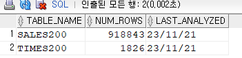
select  /*+ gather_plan_statistics leading(t s) use_nl(s) */ t.calendar_year, sum(amount_sold)
   from sales200 s, times200
   t -- times는 1826건, sales는 918843건
   where s.time_id = t.time_id
     and t.week_ending_day_id =1582 --7건!
   group by  t.calendar_year;

SELECT *
FROM TABLE(dbms_xplan.display_cursor(null,null,'ALLSTATS LAST'));

------------------------------------------------------------------------------------------------------------------------------
| Id  | Operation           | Name     | Starts | E-Rows | A-Rows |   A-Time   | Buffers | Reads  |  OMem |  1Mem | Used-Mem |
------------------------------------------------------------------------------------------------------------------------------
|   0 | SELECT STATEMENT    |          |      1 |        |      1 |00:00:01.72 |   31107 |  31024 |       |       |          |
|   1 |  HASH GROUP BY      |          |      1 |  11566 |      1 |00:00:01.72 |   31107 |  31024 |  1399K|  1399K|  487K (0)|
|   2 |   NESTED LOOPS      |          |      1 |  11566 |   6203 |00:00:00.13 |   31107 |  31024 |       |       |          |
|*  3 |    TABLE ACCESS FULL| TIMES200 |      1 |      7 |      7 |00:00:00.01 |      55 |      0 |       |       |          |
|*  4 |    TABLE ACCESS FULL| SALES200 |      7 |   1652 |   6203 |00:00:00.82 |   31052 |  31024 |       |       |          |
------------------------------------------------------------------------------------------------------------------------------
➡️ 튜닝전은 버퍼의 갯수가 50만개이고 튜닝 후는 3만으로 줄었다.
💡 특급 db 엔지니어들의 튜닝 방법 TIP!
select  /*+ gather_plan_statistics leading(s t) use_nl(t) */ t.calendar_year, sum(amount_sold)
   from sales200 s, times200 t
   where s.time_id = t.time_id
     and t.week_ending_day_id =1582
   group by  t.calendar_year;
-- 아래 통계정보 수집을 해야 num_rows와 last_analyzed가 나온다. 일할 때 null이라고 막 하지말고 해도되는지 물어봐야함 exec dbms_stats.gather_table_stats('SCOTT', 'SALES200'); exec dbms_stats.gather_table_stats('SCOTT', 'TIMES200'); select table_name, num_rows, last_analyzed from user_tables where table_name in ('SALES200','TIMES200');
-- 만약 week_ending_day_id 여기에 인덱스가 있으면 인덱스를 이용한다.
select /*+ index_ffs(t times200_indx2) parallel_index(t,times200_indx2,4) */ count(*)
 from times200 t
 where week_ending_day_id =1582;
✔️ 위처럼 하고 튜닝 수행 !
문제11. 아래의 SQL을 튜닝하기
create table customers200
as
select * from sh.customers ;
-- 튜닝전
select /*+ leading(s c) use_nl(c) */ count(*)
from sales200 s, customers200 c
where s.cust_id = c.cust_id
and c.country_id = 52790
and s.time_id between to_date('1999/01/01','YYYY/MM/DD')
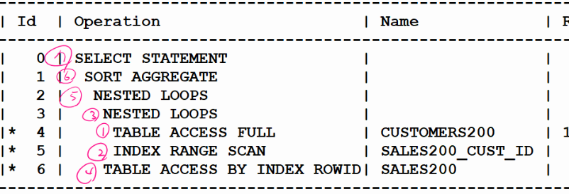
and to_date('1999/12/31','YYYY/MM/DD'); exec dbms_stats.gather_table_stats('SCOTT', 'SALES200'); exec dbms_stats.gather_table_stats('SCOTT', 'CUSTOMERS200'); -- 건수 확인 select table_name, num_rows, last_analyzed from user_tables where table_name in ('SALES200','CUSTOMERS200'); TABLE_NAME NUM_ROWS LAST_ANA ------------------------------ ---------- -------- CUSTOMERS200 54288 23/11/21 SALES200 918843 23/11/21 -- 튜닝 후 (인덱스를 만들어야 빨라서 인덱스를 만들었다.) create index sales200_cust_id on sales200(cust_id); select /*+ gather_plan_statistics leading(c s) use_nl(s) index(s sales200_cust_id) */ count(*) from sales200 s, customers200 c where s.cust_id = c.cust_id and c.country_id = 52790 -- 1만 8천건 and s.time_id between to_date('1999/01/01','YYYY/MM/DD') and to_date('1999/12/31','YYYY/MM/DD'); -- 247945건 SELECT * FROM TABLE(dbms_xplan.display_cursor(null,null,'ALLSTATS LAST')); --------------------------------------------------------------------------------------------------------------------- | Id | Operation | Name | Starts | E-Rows | A-Rows | A-Time | Buffers | Reads | --------------------------------------------------------------------------------------------------------------------- | 0 | SELECT STATEMENT | | 1 | | 1 |00:00:03.05 | 429K| 1413 | | 1 | SORT AGGREGATE | | 1 | 1 | 1 |00:00:03.05 | 429K| 1413 | | 2 | NESTED LOOPS | | 1 | 93234 | 131K|00:00:03.44 | 429K| 1413 | | 3 | NESTED LOOPS | | 1 | 371K| 487K|00:00:01.02 | 36648 | 1413 | |* 4 | TABLE ACCESS FULL | CUSTOMERS200 | 1 | 2857 | 18158 |00:00:00.04 | 1415 | 1413 | |* 5 | INDEX RANGE SCAN | SALES200_CUST_ID | 18158 | 130 | 487K|00:00:00.75 | 35233 | 0 | |* 6 | TABLE ACCESS BY INDEX ROWID| SALES200 | 487K| 33 | 131K|00:00:01.83 | 393K| 0 | ---------------------------------------------------------------------------------------------------------------------
➡️ 순서 설명!
1. customers table에서 country_id가 52790인 데이터를 검색해서 1만8천건의 데이터를 엑세스 한다. (full table scan을 했다)
2. 1번에서 찾은 1만8천건의 데이터를 가지고 조인하기 위해 cust_id 데이터를 하나씩 sales200 테이블에 cust_id를 찾아서 조인한다. 이 때 조인할때는sales200_cust_id인덱스를 통해 해당 데이터를 찾아 조인한다.➡️ 튜닝 전 SQL은 너무 오래 실행돼서 그냥 꺼버렸음...! 이것이 nested loop join의 단점!
속도를 높이려면 조인 연결고리 컬럼에 인덱스가 있어야한다. full table scan을 할거라면 hash join이 더 좋은 성능을 보이지만, hash join은 오라클 메모리를 사용하는 조인이라서 막 사용할수가 없다. oltp
문제12. 아래 SQL에 customers200 테이블의 country_id에 인덱스를 생성하면 더 검색속도가 빨라지는지 확인해보기 (위 문제 1번 순서가 full table scan하지 않게 하기위해)
✔️ SQL trace 만들기
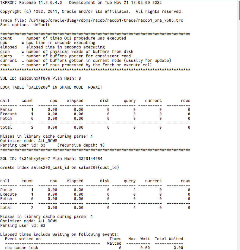
@t
-- 튜닝전 SQL 수행
select  /*+ gather_plan_statistics leading(c s) use_nl(s) index(s sales200_cust_id) */  count(*)
   from  sales200   s, customers200  c
   where  s.cust_id = c.cust_id
     and  c.country_id = 52790
     and  s.time_id between  to_date('1999/01/01','YYYY/MM/DD')
                        and  to_date('1999/12/31','YYYY/MM/DD');

-- 인덱스 만들고
create index customers200_country_id on customers200(country_id);

-- 튜닝후 SQL 수행
select  /*+ gather_plan_statistics leading(c s) use_nl(s) index(s sales200_cust_id) index(c customers200_country_id) */  count(*)
   from  sales200   s, customers200  c
   where  s.cust_id = c.cust_id
     and  c.country_id = 52790
     and  s.time_id between  to_date('1999/01/01','YYYY/MM/DD')
                        and  to_date('1999/12/31','YYYY/MM/DD');
@tf
@trace_file
TRACE_FILE_NAME
--------------------------------------------------------------------------------
/u01/app/oracle/diag/rdbms/racdb/racdb1/trace/racdb1_ora_7585.trc
@tk
✏️ Hash join (use_hash())
💡 hash join은 해쉬 알고리즘을 사용하고있는 해쉬 함수를 이용해서 메모리에 올라온 데이터를 찾아 조인하는 조인방법이다 data를 메모리에 올려놓고 메모리에서 조인하는 조인 방법이다!
select /*+ gather_plan_statistics leading(d e) use_hash(e) */ e.ename, d.loc
from emp e, dept d
where e.deptno=d.deptno;
----------------------------------------------------------------------------------------------------------------
| Id | Operation | Name | Starts | E-Rows | A-Rows | A-Time | Buffers | OMem | 1Mem | Used-Mem |
----------------------------------------------------------------------------------------------------------------
| 0 | SELECT STATEMENT | | 1 | | 14 |00:00:00.01 | 14 | | | |
|* 1 | HASH JOIN | | 1 | 14 | 14 |00:00:00.01 | 14 | 1696K| 1696K| 1027K (0)|
| 2 | TABLE ACCESS FULL| DEPT | 1 | 4 | 4 |00:00:00.01 | 7 | | | |
| 3 | TABLE ACCESS FULL| EMP | 1 | 14 | 14 |00:00:00.01 | 7 | | | |
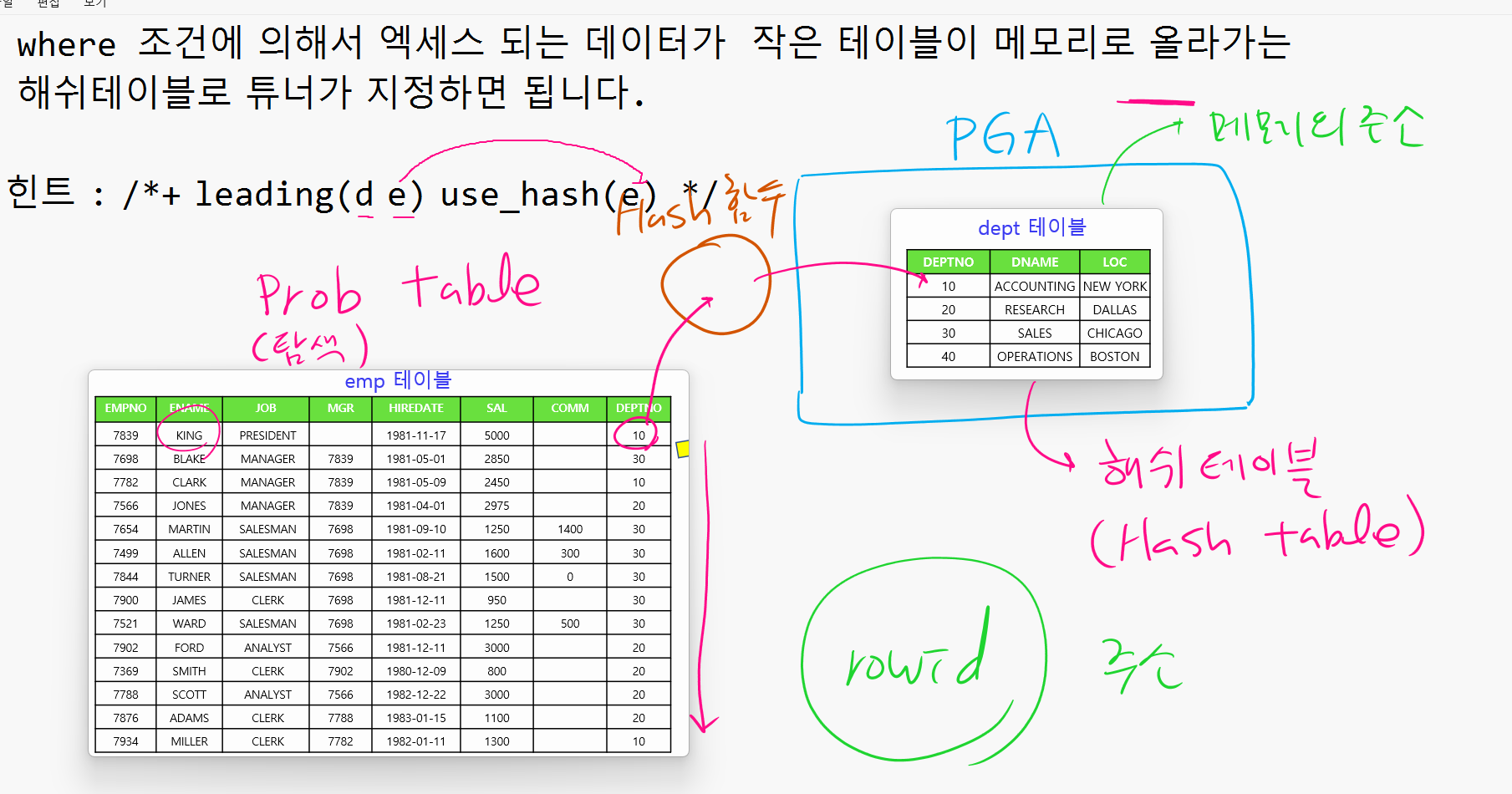
----------------------------------------------------------------------------------------------------------------➡️ 디스크에 데이터가 있을때는 로우아이디로 주소를 찾았는데 메모리에 있을때는 주소가 바뀐다. 메모리의 주소로! 그래서 중간에 있는 hash함수를 이용해서 주소를 알아내서 찾는다.
➡️ prob 테이블의 데이터를 탐색하면서 연결고리가 되는 키 컬럼의 데치터를 메모리에 올린 해쉬 테이블과 조인하는 방법!
➡️ 메모리에 테이블을 올려놓고 조인하므로 속도가 빠르다. 해쉬조인도 조인 순서가 중요한데, 작은 테이블 또는 where절 조건에 의해 생성되는 엑세스 되는 데이터가 작은 테이블이 메모리로 올라가는 해쉬 테이블로 튜너가 지정하면 된다.
❓ 만약 큰 테이블이 메모리로 올라가면 어떻게 될까?
큰 테이블을 pga영역에 모두 구성될 수 없어서 emp 테이블의 일부분만 PGA영역으로 해쉬테이블로 올라간다. 그렇다면 나머지는 temp tablespace에 나머지 데이터를 저장한다. 이렇게 되면 disk i/o가 빈번하게 일어난다. (성능 느려짐)
문제1. emp 테이블을 해시 테이블로 구성하고 dept테이블을 prob 테이블로 구성해서 해쉬조인을 하는 실행계획이 나오게 아래 SQL에 힌트를 주기
                                     조인순서      조인방법
select  /*+ gather_plan_statistics leading(d e) use_hash(e) */ e.ename, d.loc
  from emp e, dept d
  where e.deptno=d.deptno;

----------------------------------------------------------------------------------------------------------------
| Id  | Operation          | Name | Starts | E-Rows | A-Rows |   A-Time   | Buffers |  OMem |  1Mem | Used-Mem |
----------------------------------------------------------------------------------------------------------------
|   0 | SELECT STATEMENT   |      |      1 |        |     14 |00:00:00.01 |      14 |       |       |          |
|*  1 |  HASH JOIN         |      |      1 |     14 |     14 |00:00:00.01 |      14 |  1696K|  1696K|  949K (0)|
|   2 |   TABLE ACCESS FULL| DEPT |      1 |      4 |      4 |00:00:00.01 |       7 |       |       |          |
|   3 |   TABLE ACCESS FULL| EMP  |      1 |     14 |     14 |00:00:00.01 |       7 |       |       |          |
----------------------------------------------------------------------------------------------------------------
➡️
leading(d e b) use_hash(e) use_hash(b)만약 힌트를 이렇게 주었다면 dept -> emp -> bonus 테이블 순으로 조인하는데, dept,emp를 hash join하고 두개를 해쉬조인한 결과를 가지고 bonus와 hash join을 해라 라는 뜻
➡️leading(d e s) use_hash(e) use_nl(s)dept -> emp -> salgrade 순으로 조인하는데 dept와 emp를 해쉬조인하고 2개를 해쉬조인한 결과와 salgrade를 조인할 때는 mested loop조인을 해라 라는 뜻
문제2. 아래의 SQL을 해쉬조인하는데 해쉬 테이블과 PROB 테이블을 결정하는 힌트를 주고 해쉬조인하기
select e.ename, d.loc
  from emp e, dept d
  where e.deptno=d.deptno
  and e.job='SALESMAN'
  and d.loc='CHICAGO';

-- 조건절 건수 확인
select count(*) from dept where loc='CHICAGO'; -- 1개
select count(*) from dept where job='SALESMAN'; -- 4개
⭐ 테이블이 작다고 무조건 해쉬 테이블로 구성되는것은 아니고 where절 조건에 의해 엑세스 되는 건수가 작은 테이블쪽을 hash table로 구성하면 된다!
select /*+ gather_plan_statistics leading(d e) use_hash(e) */ e.ename, d.loc
  from emp e, dept d
  where e.deptno=d.deptno
  and e.job='SALESMAN'
  and d.loc='CHICAGO';

----------------------------------------------------------------------------------------------------------------
| Id  | Operation          | Name | Starts | E-Rows | A-Rows |   A-Time   | Buffers |  OMem |  1Mem | Used-Mem |
----------------------------------------------------------------------------------------------------------------
|   0 | SELECT STATEMENT   |      |      1 |        |      4 |00:00:00.01 |      14 |       |       |          |
|*  1 |  HASH JOIN         |      |      1 |      1 |      4 |00:00:00.01 |      14 |  1645K|  1645K|  604K (0)|
|*  2 |   TABLE ACCESS FULL| DEPT |      1 |      1 |      1 |00:00:00.01 |       7 |       |       |          |
|*  3 |   TABLE ACCESS FULL| EMP  |      1 |      4 |      4 |00:00:00.01 |       7 |       |       |          |
----------------------------------------------------------------------------------------------------------------
문제3. 아래의 SQL을 튜닝하기
create table sales300
 as
  select * from sh.sales;

create table customers300
 as
  select * from sh.customers;
✔️ 튜닝 전
select  /*+ gather_plan_statistics leading(s c) use_nl(c) */  count(*)
    from  sales300   s, customers300  c
    where  s.cust_id = c.cust_id
      and  c.country_id = 52790
     and  s.time_id between  to_date('1999/01/01','YYYY/MM/DD')
                        and  to_date('1999/12/31','YYYY/MM/DD');
✔️ 튜닝 후
-- customers를 먼저 읽어야 하므로 !
select  /*+ gather_plan_statistics leading(c s) use_hash(s) */  count(*)
    from  sales300   s, customers300  c
    where  s.cust_id = c.cust_id
      and  c.country_id = 52790   -- 1만 팔천건
     and  s.time_id between  to_date('1999/01/01','YYYY/MM/DD')
                        and  to_date('1999/12/31','YYYY/MM/DD'); --24만건

----------------------------------------------------------------------------------------------------------------------------------
| Id  | Operation           | Name         | Starts | E-Rows | A-Rows |   A-Time   | Buffers | Reads  |  OMem |  1Mem | Used-Mem |
----------------------------------------------------------------------------------------------------------------------------------
|   0 | SELECT STATEMENT    |              |      1 |        |      1 |00:00:00.42 |    5852 |   5845 |       |       |          |
|   1 |  SORT AGGREGATE     |              |      1 |      1 |      1 |00:00:00.42 |    5852 |   5845 |       |       |          |
|*  2 |   HASH JOIN         |              |      1 |    267K|    131K|00:00:00.24 |    5852 |   5845 |  2484K|  2484K| 2201K (0)|
|*  3 |    TABLE ACCESS FULL| CUSTOMERS300 |      1 |  16881 |  18158 |00:00:00.01 |    1416 |   1413 |       |       |          |
|*  4 |    TABLE ACCESS FULL| SALES300     |      1 |    267K|    247K|00:00:00.13 |    4436 |   4432 |       |       |          |
----------------------------------------------------------------------------------------------------------------------------------
문제4. 아래의 조인 순서를 sales300 -> customers300이 되게 하기
select  /*+ gather_plan_statistics leading(s c) use_hash(c) */  count(*)
    from  sales300   s, customers300  c
    where  s.cust_id = c.cust_id
      and  c.country_id = 52790   -- 1만 팔천건
     and  s.time_id between  to_date('1999/01/01','YYYY/MM/DD')
                        and  to_date('1999/12/31','YYYY/MM/DD');

----------------------------------------------------------------------------------------------------------------------------------
| Id  | Operation           | Name         | Starts | E-Rows | A-Rows |   A-Time   | Buffers | Reads  |  OMem |  1Mem | Used-Mem |
----------------------------------------------------------------------------------------------------------------------------------
|   0 | SELECT STATEMENT    |              |      1 |        |      1 |00:00:00.35 |    5852 |   5845 |       |       |          |
|   1 |  SORT AGGREGATE     |              |      1 |      1 |      1 |00:00:00.35 |    5852 |   5845 |       |       |          |
|*  2 |   HASH JOIN         |              |      1 |    267K|    131K|00:00:00.31 |    5852 |   5845 |    10M|  3056K|   16M (0)|
|*  3 |    TABLE ACCESS FULL| SALES300     |      1 |    267K|    247K|00:00:00.09 |    4436 |   4432 |       |       |          |
|*  4 |    TABLE ACCESS FULL| CUSTOMERS300 |      1 |  16881 |  18158 |00:00:00.01 |    1416 |   1413 |       |       |          |
----------------------------------------------------------------------------------------------------------------------------------
➡️ 버퍼의 갯수는 차이가 보이지 않지만 메모리 사용량이 차이가 난다. Used-Mem 를 보면 cunstomers300을 메모리로 올렸을 때는 2201K 지만 saels300을 올렸을 때는 16M이다.
❓hash join은 언제 사용할 때 유리할까
1. 수행 빈도가 낮은 쿼리문
ex) 실시간으로 주문이 들어오는 OLTP 시스템에는 해쉬조인 사용이 부적절하다.
    서로 메모리에 해쉬테이블을 구성하려고 경합을 일으키면 안되므로!
    데이터 분석을 위해 쿼리를 하는 DW쪽 쿼리문에 유리하다.
2. 쿼리의 수행시간이 오래 걸리는 SQL
3. 대용량 테이블을 조인할 때 주로 사용⭐ OLTP ()환경 즉 짧은 수행시간이 걸리면서 수행빈도가 높은 SQL이 많이 수행되는 환경에서 1초 걸리는 쿼리를 0.1초 단축시킬 목적으로 해쉬조인을 사용하는것은 자제해야한다.
🚨 hash join을 할 때 주의사항
- 인덱스 스캔이 되면 오히려 성능이 떨어진다. full table scan이 되어져야 한다.
- 작은 테이블이거나 where조건에 의해 액세스 되는 건수가 작은 테이블이 해쉬 테이블로 구성되어져야 한다!
문제5. 아래의 인덱스를 생성하고 아래 SQL의 실제 실행계획을 확인해보기
create index sales300_cust_id on sales300(cust_id);

select  /*+ gather_plan_statistics index(s sales300_cust_id) leading(c s) use_hash(s) */  count(*)
   from  sales300   s, customers300  c
   where  s.cust_id = c.cust_id
     and  c.country_id = 52790
     and  s.time_id between  to_date('1999/01/01','YYYY/MM/DD')
                        and  to_date('1999/12/31','YYYY/MM/DD');

------------------------------------------------------------------------------------------------------------------------------------------------
| Id  | Operation                     | Name             | Starts | E-Rows | A-Rows |   A-Time   | Buffers | Reads  |  OMem |  1Mem | Used-Mem |
------------------------------------------------------------------------------------------------------------------------------------------------
|   0 | SELECT STATEMENT              |                  |      1 |        |      1 |00:00:01.77 |     748K|   7514 |       |       |          |
|   1 |  SORT AGGREGATE               |                  |      1 |      1 |      1 |00:00:01.77 |     748K|   7514 |       |       |          |
|*  2 |   HASH JOIN                   |                  |      1 |    267K|    131K|00:00:01.31 |     748K|   7514 |  2484K|  2484K| 2245K (0)|
|*  3 |    TABLE ACCESS FULL          | CUSTOMERS300     |      1 |  16881 |  18158 |00:00:00.01 |    1416 |   1413 |       |       |          |
|*  4 |    TABLE ACCESS BY INDEX ROWID| SALES300         |      1 |    267K|    247K|00:00:00.91 |     747K|   6101 |       |       |          |
|   5 |     INDEX FULL SCAN           | SALES300_CUST_ID |      1 |    845K|    918K|00:00:00.40 |    1949 |   1948 |       |       |          |
------------------------------------------------------------------------------------------------------------------------------------------------
7십4만8천
✔️ 튜닝 후
select  /*+ gather_plan_statistics full(s) full(s) leading(c s) use_hash(s) */  count(*)
   from  sales300   s, customers300  c
   where  s.cust_id = c.cust_id
     and  c.country_id = 52790
     and  s.time_id between  to_date('1999/01/01','YYYY/MM/DD')
                        and  to_date('1999/12/31','YYYY/MM/DD');

----------------------------------------------------------------------------------------------------------------------------------
| Id  | Operation           | Name         | Starts | E-Rows | A-Rows |   A-Time   | Buffers | Reads  |  OMem |  1Mem | Used-Mem |
----------------------------------------------------------------------------------------------------------------------------------
|   0 | SELECT STATEMENT    |              |      1 |        |      1 |00:00:00.14 |    5856 |   1413 |       |       |          |
|   1 |  SORT AGGREGATE     |              |      1 |      1 |      1 |00:00:00.14 |    5856 |   1413 |       |       |          |
|*  2 |   HASH JOIN         |              |      1 |    267K|    131K|00:00:00.14 |    5856 |   1413 |  2484K|  2484K| 2245K (0)|
|*  3 |    TABLE ACCESS FULL| CUSTOMERS300 |      1 |  16881 |  18158 |00:00:00.03 |    1416 |   1413 |       |       |          |
|*  4 |    TABLE ACCESS FULL| SALES300     |      1 |    267K|    247K|00:00:00.03 |    4440 |      0 |       |       |          |
----------------------------------------------------------------------------------------------------------------------------------
➡️ 버퍼의 갯수가 확연하게 줄어들었다.
문제6. 아래의 SQL을 튜닝하기
create  table  products300
  as
   select  * from  sh.products;

-- 튜닝전
select  /*+ gather_plan_statistics leading(s p) use_hash(p) */
                   p.prod_name, sum(s.amount_sold)
              from  sales300  s, products300  p
              where  s.prod_id = p.prod_id
               and  p.prod_name   like 'Deluxe%'
              group  by  p.prod_name;

------------------------------------------------------------------------------------------------------------------------
| Id  | Operation           | Name        | Starts | E-Rows | A-Rows |   A-Time   | Buffers |  OMem |  1Mem | Used-Mem |
------------------------------------------------------------------------------------------------------------------------
|   0 | SELECT STATEMENT    |             |      1 |        |      1 |00:00:00.11 |    4444 |       |       |          |
|   1 |  HASH GROUP BY      |             |      1 |  14329 |      1 |00:00:00.11 |    4444 |  1827K|  1462K|  541K (0)|
|*  2 |   HASH JOIN         |             |      1 |  14329 |  12837 |00:00:00.11 |    4444 |    44M|     9M|   65M (0)|
|   3 |    TABLE ACCESS FULL| SALES300    |      1 |    845K|    918K|00:00:00.08 |    4440 |       |       |          |
|*  4 |    TABLE ACCESS FULL| PRODUCTS300 |      1 |      1 |      1 |00:00:00.01 |       4 |       |       |          |
------------------------------------------------------------------------------------------------------------------------
✔️ 튜닝 후
: 작은 테이블인 products300를 앞에!select /*+ gather_plan_statistics leading(p s) use_hash(s) */ p.prod_name, sum(s.amount_sold) from sales300 s, products300 p where s.prod_id = p.prod_id and p.prod_name like 'Deluxe%' group by p.prod_name; ------------------------------------------------------------------------------------------------------------------------ | Id | Operation | Name | Starts | E-Rows | A-Rows | A-Time | Buffers | OMem | 1Mem | Used-Mem | ------------------------------------------------------------------------------------------------------------------------ | 0 | SELECT STATEMENT | | 1 | | 1 |00:00:00.07 | 4444 | | | | | 1 | HASH GROUP BY | | 1 | 14329 | 1 |00:00:00.07 | 4444 | 1827K| 1462K| 782K (0)| |* 2 | HASH JOIN | | 1 | 14329 | 12837 |00:00:00.39 | 4444 | 1451K| 1451K| 411K (0)| |* 3 | TABLE ACCESS FULL| PRODUCTS300 | 1 | 1 | 1 |00:00:00.01 | 4 | | | | | 4 | TABLE ACCESS FULL| SALES300 | 1 | 845K| 918K|00:00:00.08 | 4440 | | | | ------------------------------------------------------------------------------------------------------------------------➡️ 버퍼의 갯수는 차이가 없지만 속도가 달랐다. 작은 테이블이 메모리에 올라가야한다!!
문제7. 아래의 SQL을 nested loop 조인으로 유도하는데 인덱스가 필요하면 자유롭게 인덱스를 생성해서 제일 좋은 결과로 출력되게 하기
select  /*+ gather_plan_statistics leading(p s) use_nl(s) */
                   p.prod_name, sum(s.amount_sold)
              from  sales300  s, products300  p
              where  s.prod_id = p.prod_id
               and  p.prod_name   like 'Deluxe%'
              group  by  p.prod_name;
✅ index를 s.prod_id 쪽에 걸어주면 된다. 풀테이블 스캔 하지 않도록!
create index sales300_prod_id on sales300(prod_id);
select /*+ gather_plan_statistics leading(p s) use_nl(s) index(s sales300_prod_id) */
p.prod_name, sum(s.amount_sold)
from sales300 s, products300 p
where s.prod_id = p.prod_id
and p.prod_name like 'Deluxe%'
group by p.prod_name;
---------------------------------------------------------------------------------------------------------------------------------------
| Id | Operation | Name | Starts | E-Rows | A-Rows | A-Time | Buffers | OMem | 1Mem | Used-Mem |
---------------------------------------------------------------------------------------------------------------------------------------
| 0 | SELECT STATEMENT | | 1 | | 1 |00:00:00.01 | 216 | | | |
| 1 | HASH GROUP BY | | 1 | 14329 | 1 |00:00:00.01 | 216 | 1827K| 1462K| 808K (0)|
| 2 | NESTED LOOPS | | 1 | 14329 | 12837 |00:00:00.01 | 216 | | | |
| 3 | NESTED LOOPS | | 1 | 14329 | 12837 |00:00:00.01 | 32 | | | |
|* 4 | TABLE ACCESS FULL | PRODUCTS300 | 1 | 1 | 1 |00:00:00.01 | 4 | | | |
|* 5 | INDEX RANGE SCAN | SALES300_PROD_ID | 1 | 14329 | 12837 |00:00:00.01 | 28 | | | |
| 6 | TABLE ACCESS BY INDEX ROWID| SALES300 | 12837 | 14329 | 12837 |00:00:00.01 | 184 | | | |
---------------------------------------------------------------------------------------------------------------------------------------
-- 위에 full table scan이 나오지 않도록 prod_name에 인덱스 걸기
create index products300_prod_name on products300(prod_name);
select /*+ gather_plan_statistics leading(p s) use_nl(s) index(s sales300_prod_id) index(p products300_prod_name) */
p.prod_name, sum(s.amount_sold)
from sales300 s, products300 p
where s.prod_id = p.prod_id
and p.prod_name like 'Deluxe%'
group by p.prod_name;
------------------------------------------------------------------------------------------------------------------
| Id | Operation | Name | Starts | E-Rows | A-Rows | A-Time | Buffers |
------------------------------------------------------------------------------------------------------------------
| 0 | SELECT STATEMENT | | 1 | | 1 |00:00:00.01 | 214 |
| 1 | SORT GROUP BY NOSORT | | 1 | 14329 | 1 |00:00:00.01 | 214 |
| 2 | NESTED LOOPS | | 1 | 14329 | 12837 |00:00:00.02 | 214 |
| 3 | NESTED LOOPS | | 1 | 14329 | 12837 |00:00:00.01 | 30 |
| 4 | TABLE ACCESS BY INDEX ROWID| PRODUCTS300 | 1 | 1 | 1 |00:00:00.01 | 2 |
|* 5 | INDEX RANGE SCAN | PRODUCTS300_PROD_NAME | 1 | 1 | 1 |00:00:00.01 | 1 |
|* 6 | INDEX RANGE SCAN | SALES300_PROD_ID | 1 | 14329 | 12837 |00:00:00.01 | 28 |
| 7 | TABLE ACCESS BY INDEX ROWID | SALES300 | 12837 | 14329 | 12837 |00:00:00.01 | 184 |
------------------------------------------------------------------------------------------------------------------
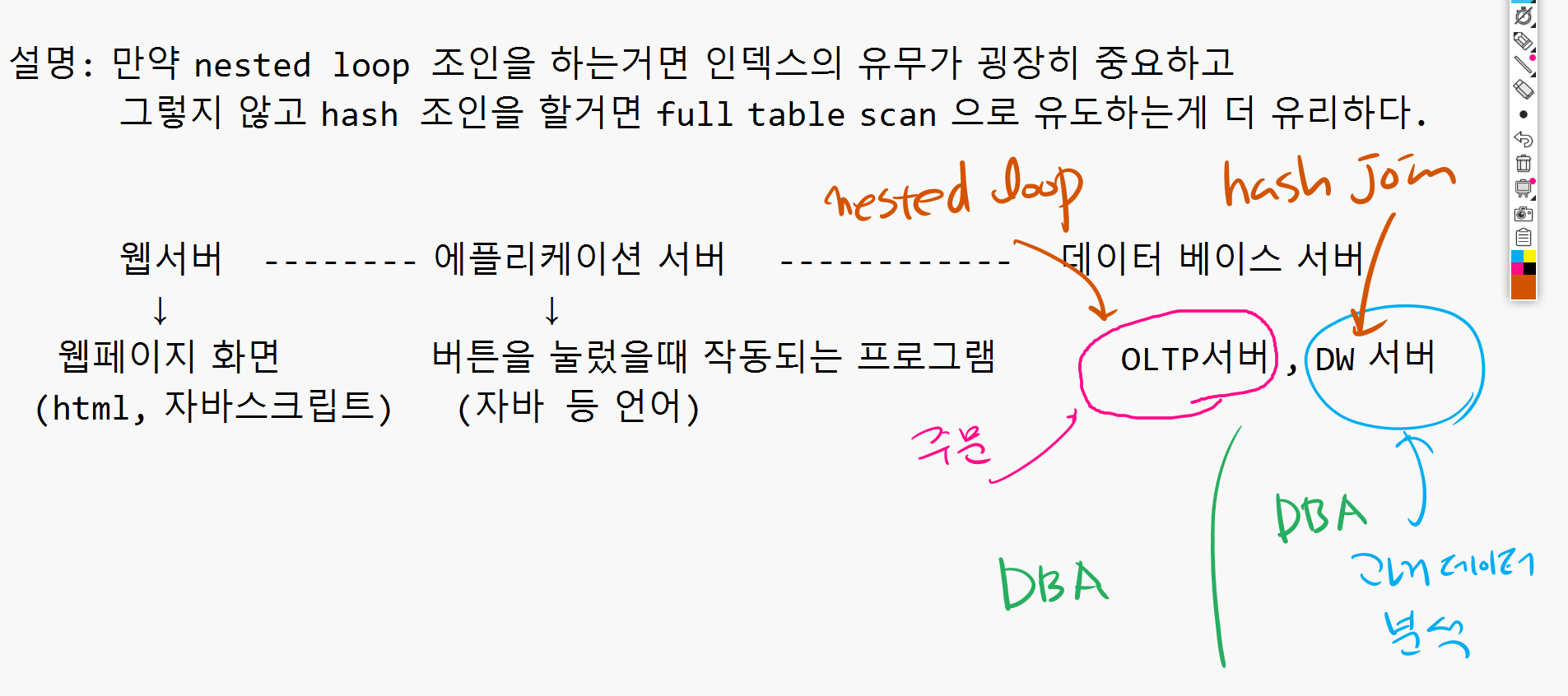
-- full table scan이 사라졌다.➡️ 만약 nested loop join을 하는거면 인덱스의 유무가 굉장히 중요하고 hash join을 할거면 full table scan으로 유도하는것이 더 유리하다!
       웹서버 --------------- 애플리케이션 서버 --------------- 데이터 베이스 서버
    웹페이지 화면        버튼을 눌렀을 때 작동되는 프로그램         OLTP서버, DW서버
 (html,자바스크립트)             (자바 등 언어)
⭐ OLTP 서버는 nested loop join , DW 서버는 hash join
문제8. EMP, SALGRADE를 조인해서 이름, 월급, 급여등급을 출력하는데 조인방법이 hash조인이 되도록
select /*+ gather_plan_statistics leading(s e) use_hash(e) */ e.ename, e.sal, s.grade
 from emp e, salgrade s
 where e.sal between s.losal and s.hisal ;

-----------------------------------------------------------------------------------------
| Id  | Operation          | Name     | Starts | E-Rows | A-Rows |   A-Time   | Buffers |
-----------------------------------------------------------------------------------------
|   0 | SELECT STATEMENT   |          |      1 |        |     14 |00:00:00.01 |      42 |
|   1 |  NESTED LOOPS      |          |      1 |      1 |     14 |00:00:00.01 |      42 |
|   2 |   TABLE ACCESS FULL| SALGRADE |      1 |      5 |      5 |00:00:00.01 |       7 |
|*  3 |   TABLE ACCESS FULL| EMP      |      5 |      1 |     14 |00:00:00.01 |      35 |
-----------------------------------------------------------------------------------------
❓ hash join힌트를 주었는데 왜
NESTED LOOPS????where절의 조인 연결고리가
=가 아니면 해쉬조인을 할 수 없다.: 2개의 테이블이 대용량 테이블이면 해쉬조인을 해야하는데 위와 같이 해쉬조인을 할 수 없다면 sort merge join으로 해결하면 된다.
✏️ sort merge join (use_merge)
💡 조인하려는 데이터의 양이 많을 때 유리한 조인 방법. 조인하려는 테이블의 키 컬럼을 미리 정렬해놓고 빠르게 조인하는 조인 방법이다!
select /*+ gather_plan_statistics leading(d e) use_merge(e) */ e.ename, d.loc, e.deptno
  from emp e, dept d
  where d.deptno=e.deptno;

-----------------------------------------------------------------------------------------------------------------
| Id  | Operation           | Name | Starts | E-Rows | A-Rows |   A-Time   | Buffers |  OMem |  1Mem | Used-Mem |
-----------------------------------------------------------------------------------------------------------------
|   0 | 6SELECT STATEMENT    |      |      1 |        |     14 |00:00:00.01 |      14 |       |       |          |
|   1 | 5 MERGE JOIN         |      |      1 |     14 |     14 |00:00:00.01 |      14 |       |       |          |
|   2 | 2  SORT JOIN         |      |      1 |      4 |      4 |00:00:00.01 |       7 |  2048 |  2048 | 2048  (0)|
|   3 | 1   TABLE ACCESS FULL| DEPT |      1 |      4 |      4 |00:00:00.01 |       7 |       |       |          |
|*  4 | 4  SORT JOIN         |      |      4 |     14 |     14 |00:00:00.01 |       7 |  2048 |  2048 | 2048  (0)|
|   5 | 3   TABLE ACCESS FULL| EMP  |      1 |     14 |     14 |00:00:00.01 |       7 |       |       |          |
----------------------------------------------------------------------------------------------------------------- 
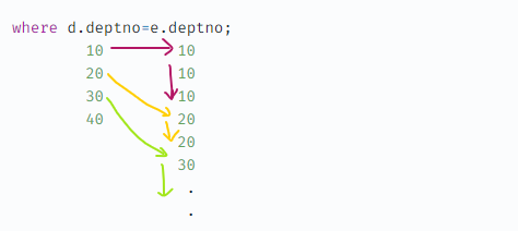
➡️ 연결고리가 되는 부서번호를 정렬해 놓고 쫙 조인하는 것 !!
문제9. 아래의 SQL을 sort merge join으로 유도하기
select /*+ gather_plan_statistics leading(s e) use_merge(e) */ e.ename, e.sal, s.grade
 from emp e, salgrade s
 where e.sal between s.losal and s.hisal ;

----------------------------------------------------------------------------------------------------------------------
| Id  | Operation            | Name     | Starts | E-Rows | A-Rows |   A-Time   | Buffers |  OMem |  1Mem | Used-Mem |
----------------------------------------------------------------------------------------------------------------------
|   0 | SELECT STATEMENT     |          |      1 |        |     14 |00:00:00.01 |      14 |       |       |          |
|   1 |  MERGE JOIN          |          |      1 |      1 |     14 |00:00:00.01 |      14 |       |       |          |
|   2 |   SORT JOIN          |          |      1 |      5 |      5 |00:00:00.01 |       7 |  2048 |  2048 | 2048  (0)|
|   3 |    TABLE ACCESS FULL | SALGRADE |      1 |      5 |      5 |00:00:00.01 |       7 |       |       |          |
|*  4 |   FILTER             |          |      5 |        |     14 |00:00:00.01 |       7 |       |       |          |
|*  5 |    SORT JOIN         |          |      5 |     14 |     40 |00:00:00.01 |       7 |  2048 |  2048 | 2048  (0)|
|   6 |     TABLE ACCESS FULL| EMP      |      1 |     14 |     14 |00:00:00.01 |       7 |       |       |          |
----------------------------------------------------------------------------------------------------------------------
문제10. 아래의 SQL을 3가지 조인 방법으로 각각 유도해보기
select e.ename, e.sal, d.loc
  from emp e, dept d
  where e.deptno=d.deptno;
✔️ dept -> emp (nested loop join)
select /*+ gather_plan_statistics leading(d e) use_nl(e) */ e.ename, e.sal, d.loc
  from emp e, dept d
  where e.deptno=d.deptno;
✔️ dept -> emp (hash join)
select /*+ gather_plan_statistics leading(d e) use_hash(e) */ e.ename, e.sal, d.loc
  from emp e, dept d
  where e.deptno=d.deptno;
✔️ dept -> emp (sort merge join)
select /*+ gather_plan_statistics leading(d e) use_merge(e) */ e.ename, e.sal, d.loc
  from emp e, dept d
  where e.deptno=d.deptno;
✏️ 조인 순서의 중요성
💡 조인 순서에 따라 수행 성능이 달라질 수 있다. 조인 순서는 조인하려는 시도횟수가 적은 테이블을 driving 테이블로 선정해서 조인 순서를 고려하는것이 중요하다.
문제1. 아래의 SQL의 조인순서가 emp->dept->salgrade 순서가 되게 하기. (조인 방법은 모두 nested loop join)
select e.ename, e.sal, d.loc, s.grade
  from emp e, dept d, salgrade s
  where e.deptno=d.deptno
    and e.sal between s.losal and s.hisal ;
✔️ 답
select /*+ gather_plan_statistics leading(e d s) use_nl(d) use_nl(s) */ e.ename, e.sal, d.loc, s.grade
  from emp e, dept d, salgrade s
  where e.deptno=d.deptno
    and e.sal between s.losal and s.hisal ;

------------------------------------------------------------------------------------------
| Id  | Operation           | Name     | Starts | E-Rows | A-Rows |   A-Time   | Buffers |
------------------------------------------------------------------------------------------
|   0 | SELECT STATEMENT    |          |      1 |        |     14 |00:00:00.01 |     203 |
|   1 |  NESTED LOOPS       |          |      1 |      1 |     14 |00:00:00.01 |     203 |
|   2 |   NESTED LOOPS      |          |      1 |     14 |     14 |00:00:00.01 |     105 |
|   3 |    TABLE ACCESS FULL| EMP      |      1 |     14 |     14 |00:00:00.01 |       7 |
|*  4 |    TABLE ACCESS FULL| DEPT     |     14 |      1 |     14 |00:00:00.01 |      98 |
|*  5 |   TABLE ACCESS FULL | SALGRADE |     14 |      1 |     14 |00:00:00.01 |      98 |
------------------------------------------------------------------------------------------
➡️ emp -> dept -> salgrade 일때
emp -> dept를 먼저 조인하고 그 결과집합으로 salgrade랑 NESTED LOOPS조인을 하는 것이다.
문제2. 아래 SQL의 실행계획이 이미지와 같이 출력되게 하기 (SQLP시험)
select /*+ gather_plan_statistics leading(e d s) use_nl(d) use_nl(s) */ e.ename, e.sal, d.loc, s.grade
  from emp e, dept d, salgrade s
  where e.deptno=d.deptno
    and e.sal between s.losal and s.hisal ;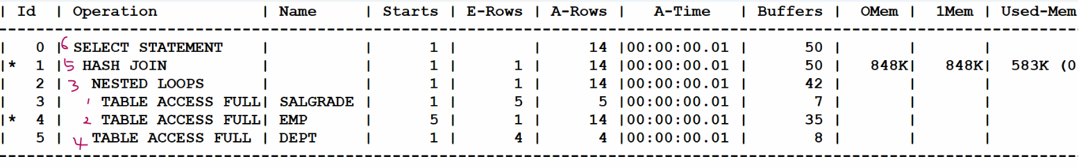
select /*+ gather_plan_statistics leading(s e d) use_nl(e) use_hash(d) */ e.ename, e.sal, d.loc, s.grade
  from emp e, dept d, salgrade s
  where e.deptno=d.deptno
    and e.sal between s.losal and s.hisal ;

---------------------------------------------------------------------------------------------------------------------
| Id  | Operation           | Name     | Starts | E-Rows | A-Rows |   A-Time   | Buffers |  OMem |  1Mem | Used-Mem |
---------------------------------------------------------------------------------------------------------------------
|   0 | SELECT STATEMENT    |          |      1 |        |     14 |00:00:00.01 |      49 |       |       |          |
|*  1 |  HASH JOIN          |          |      1 |      1 |     14 |00:00:00.01 |      49 |  1421K|  1421K|  648K (0)|
|   2 |   NESTED LOOPS      |          |      1 |      1 |     14 |00:00:00.01 |      42 |       |       |          |
|   3 |    TABLE ACCESS FULL| SALGRADE |      1 |      5 |      5 |00:00:00.01 |       7 |       |       |          |
|*  4 |    TABLE ACCESS FULL| EMP      |      5 |      1 |     14 |00:00:00.01 |      35 |       |       |          |
|   5 |   TABLE ACCESS FULL | DEPT     |      1 |      4 |      4 |00:00:00.01 |       7 |       |       |          |
---------------------------------------------------------------------------------------------------------------------
오늘의 마지막 문제 아래 SQL이 아래와 같이 실행계획이 출력될 수 있도록 하기!
select /*+ gather_plan_statistics leading(e d s) use_nl(d) use_nl(s) */ e.ename, e.sal, d.loc, s.grade
  from emp e, dept d, salgrade s
  where e.deptno=d.deptno
    and e.sal between s.losal and s.hisal ;
select /*+ gather_plan_statistics leading(e s d) use_merge(s) use_hash(d) */ e.ename, e.sal, d.loc, s.grade from emp e, dept d, salgrade s where e.deptno=d.deptno and e.sal between s.losal and s.hisal ; ----------------------------------------------------------------------------------------------------------------------- | Id | Operation | Name | Starts | E-Rows | A-Rows | A-Time | Buffers | OMem | 1Mem | Used-Mem | ----------------------------------------------------------------------------------------------------------------------- | 0 | SELECT STATEMENT | | 1 | | 14 |00:00:00.01 | 21 | | | | |* 1 | HASH JOIN | | 1 | 1 | 14 |00:00:00.01 | 21 | 1421K| 1421K| 650K (0)| | 2 | MERGE JOIN | | 1 | 1 | 14 |00:00:00.01 | 14 | | | | | 3 | SORT JOIN | | 1 | 14 | 14 |00:00:00.01 | 7 | 2048 | 2048 | 2048 (0)| | 4 | TABLE ACCESS FULL | EMP | 1 | 14 | 14 |00:00:00.01 | 7 | | | | |* 5 | FILTER | | 14 | | 14 |00:00:00.01 | 7 | | | | |* 6 | SORT JOIN | | 14 | 5 | 40 |00:00:00.01 | 7 | 2048 | 2048 | 2048 (0)| | 7 | TABLE ACCESS FULL| SALGRADE | 1 | 5 | 5 |00:00:00.01 | 7 | | | | | 8 | TABLE ACCESS FULL | DEPT | 1 | 4 | 4 |00:00:00.01 | 7 | | | | -----------------------------------------------------------------------------------------------------------------------
