
📢 개요
앞선 Data Cleansing(1), (2) 포스트에서는 데이터의 품질을 저하시키는 요인인 결측치와 이상치의 탐색 및 처리 방법에 대하여 알아보았다. 잡음(Noise) 역시 실제 데이터의 정보의 왜곡 및 간섭을 초래하는 요인에 해당하며 이는 데이터의 신뢰성을 낮추고 잘못된 의사결정으로 이어질 수 있기에 반드시 적절한 처리가 필요하다. 이번 포스트에서 잡음 처리에 대한 내용을 끝으로 Data Cleansing 내용 정리를 마무리하고자 한다.
✏️ 잡음(Noise)이란?
👉 측정된 변수에 무작위의 오류(Random Error) 또는 분산(Variance)가 존재하는 것
👉 실제로는 입력되지 않았지만 입력되었다고 잘못 판단된 값
👉 일반적으로 원인을 알 수 없는 데이터의 무작위 변동
👉 오류 및 오차 값에 의해 데이터의 경향성이 훼손됨
👉 무작위 변동의 발생 기전(mechanism)을 모르기에, 제거는 불가능하며 이를 저감(Denoising)하는 방식으로 처리해야 함
📌 잡음(Noise) vs 이상치(Outlier)
- 이상치(Outlier)
- 데이터의 무작위 변동을 초과하는 특정한 값으로 별도로 처리
- 잡음(Noise)
- 관측을 잘못하거나 시스템에서 발생하는 무작위적 오류(random error)등에 의해 발생하는 것으로 이상치를 탐지할 때 제거되어야 할 요소
잡음(Noise)은 관심이 없어 제거할 대상이지만, 이상치(Outlier)는 관심의 대상
📂 잡음(Noise) 종류
1. Gaussian Noise
👉 평균 0, 분산 1의 정규분포를 따르는 잡음
👉 이미지/영상 데이터에서 일반적으로 발생
2. Salt and Pepper Noise
👉 검은색 또는 흰색 점의 형태로 발생하는 잡음
👉 0 또는 255의 픽셀 값과 같이 뚜렷하게 잘못된 밝기 값을 갖는 Impulse Noise
👉 이미지/영상 데이터에서 일반적으로 발생
3. Uniform Noise
👉 균일한 분포를 갖는 잡음
👉 이미지/영상 데이터 전체 영역에 대해서 동일 패턴을 갖는 잡음이 일정하게 발생
4. Pink Noise
👉 특정 주파수 대역(일반적으로 낮은 주파수)에서 강하게 나타나는 잡음
👉 음향 데이터에서 일반적으로 발생
5. White Noise
👉 평균 0, 분산 의 분포를 갖는 잡음
👉 모든 주파수에서 동일 세기를 가지는, 즉 어떠한 추세(trend)를 보이지 않는 잡음
👉 패턴이 random 하기에 Random Noise라고도 함
📍예시
📚 데이터 유형별 잡음(Noise)
📅 Noise in Structured Data
👉 정형 데이터에서의 Noise는 분산(Variance) 으로 나타남
👉 통계 모델에서는 오차항(모델이 설명하지 못하는 무작위 변동) 으로 나타남
🧩 예) 단순선형회귀(Simple Linear Regression) 모델 에서의 오차항 이 Noise에 해당
📍 예시 (Reliability of Linear Regression Model by Noise)
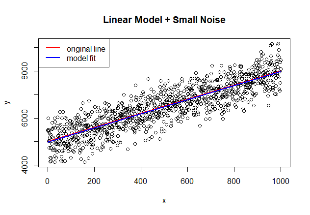
1) Linear Model + Small White Noise
# R code

set.seed(500)
noise_small<-rnorm(1000,0,500)

x<-seq(1:1000)
y<-noise_small+(5000+3*x) # adding Noise to the line Y=5000 + 3X
line<-5000+3*x

plot(x,y, main="Line + Small Noise")
lines(line, col="red", lwd=2)
legend ("topleft", legend=c("underlying line"), col=c("red"), lty=1, lwd=2)

data<-data.frame(x=x,y=y)
model<-lm(y ~ x, data)
summary(model)
# result Call: lm(formula = y ~ x, data = data) Residuals: Min 1Q Median 3Q Max -1332 -332 6 356 1387 Coefficients: Estimate Std. Error t value Pr(>|t|) (Intercept) 4.97e+03 3.16e+01 157.2 <2e-16 *** x 3.01e+00 5.47e-02 54.9 <2e-16 *** --- Signif. codes: 0 '***' 0.001 '**' 0.01 '*' 0.05 '.' 0.1 ' ' 1 Residual standard error: 500 on 998 degrees of freedom Multiple R-squared: 0.751, Adjusted R-squared: 0.751 F-statistic: 3.02e+03 on 1 and 998 DF, p-value: <2e-16
- 회귀분석 결과 추정된 편향(Intercept)와 가중치(x, 회귀계수)는 각각 4970, 3.01이며 결정계수(Adjusted R-squared)는 0.751
- Noise가 존재함에도 불구하고 추정된 선형회귀 모형의 적합도가 매우 높음을 확인 가능
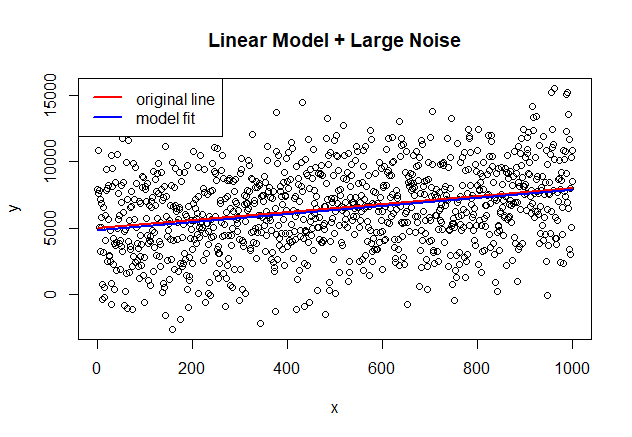
2) Linear Model + Large White Noise
# R code

set.seed(500)
noise_large<-rnorm(1000,0,3000)

x<-seq(1:1000)
y<-noise_large+(5000+3*x)
line<-5000+3*x

plot(x,y, main="Line + Large Noise")
lines(line, col="red", lwd=2)
legend ("topleft", legend=c("underlying line"), col=c("red"), lty=1, lwd=2, bg="white")

data<-data.frame(x=x,y=y)
model<-lm(y ~ x, data)
summary(model)
# result Call: lm(formula = y ~ x, data = data) Residuals: Min 1Q Median 3Q Max -7989 -1993 36 2136 8324 Coefficients: Estimate Std. Error t value Pr(>|t|) (Intercept) 4832.032 189.777 25.46 <2e-16 *** x 3.043 0.328 9.27 <2e-16 *** --- Signif. codes: 0 '***' 0.001 '**' 0.01 '*' 0.05 '.' 0.1 ' ' 1 Residual standard error: 3000 on 998 degrees of freedom Multiple R-squared: 0.0792, Adjusted R-squared: 0.0783 F-statistic: 85.9 on 1 and 998 DF, p-value: <2e-16
- 회귀분석 결과 추정된 편향(Intercept)와 가중치(x, 회귀계수)는 각각 4832, 3.04이며 결정계수(Adjusted R-squared)는 0.0783
- 회귀분석으로 추정된 선형회귀 모형의 적합도는 높으나, 결정계수 값이 Small White Noise case와 비교하였을 때 매우 낮은 결과를 보임
- 높은 적합도 결과를 통해 선형회귀 모형이 많은 양의 Noise가 존재하는 데이터임에도 불구하고 Signal을 올바르게 선택하였음을 설명 가능
- 매우 낮은 결정계수 값 결과를 통해 추정된 모형을 예측 목적으로는 사용 불가함을 확인 가능
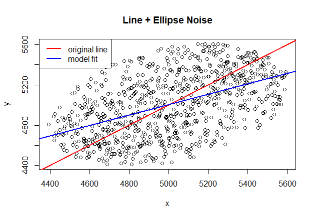
3) Linear Model + Non-White Noise
# R code

# the ellipse of noise will be centered at (5000,5000) but rotated 45 degrees to match
angle<-pi/4
a<-700
b<-500
center_x <- 5000
center_y <- 5000
angle<-pi/4
data<-data.frame(x=seq(1:noisepoints),y=noisyaxle)

# filter noise points within the ellipse
points<-data[((data$x-center_x)*cos(angle)+(data$y-center_y)*sin(angle))^2/a^2 + (-(data$x-center_x)*sin(angle)+(data$y-center_y)*cos(angle))^2/b^2 <= 1,]
plot(points, main="Line + Ellipse Noise")
lines(seq(1:noisepoints),seq(1:noisepoints), col="red", lwd=2)
legend ("topleft", legend=c("underlying line"), col=c("red"), lty=1, lwd=2, bg="white")

model<-lm(y ~ x , points)
summary(model)
# result Call: lm(formula = y ~ x, data = points) Residuals: Min 1Q Median 3Q Max -588.8 -214.2 0.5 200.9 575.8 Coefficients: Estimate Std. Error t value Pr(>|t|) (Intercept) 2.41e+03 1.58e+02 15.3 <2e-16 *** x 5.18e-01 3.16e-02 16.4 <2e-16 *** --- Signif. codes: 0 '***' 0.001 '**' 0.01 '*' 0.05 '.' 0.1 ' ' 1 Residual standard error: 266 on 801 degrees of freedom Multiple R-squared: 0.251, Adjusted R-squared: 0.251 F-statistic: 269 on 1 and 801 DF, p-value: <2e-16
- 회귀분석 결과 추정된 편향(Intercept)와 가중치(x, 회귀계수)는 각각 2410, 5.18이며 결정계수(Adjusted R-squared)는 0.251
- 추정된 선형회귀 모형의 적합도가 매우 낮음을 확인 가능
- 이는 Noise data가 White Noise가 아닌 타원의 형태로 분포를 갖는 Ellipse Noise에 해당하기에 왜곡이 발생한 것
데이터 상에 Noise가 존재한다고 할 때, Noise가 많고 적음의 정량적 수치에 따라서도 기존 데이터에 영향을 주는 정도가 상이하지만, Noise의 종류에 따라서도 실제 데이터의 분포에 미치는 영향이 크게 발생!
🖼️ Noise in Image(사진/영상) Data
👉 사진/영상 데이터에서의 Noise는 Blur, White Noise, Pink Noise, Gausian Noise 등 다양한 형태로 발생
👉 발생 주 원인으로는 이미지 획득과정에서 너무 낮은 수집된 광자의 양, 센서/렌즈 열화, 이미지 전송 중 무선 통신의 에코 및 대기왜곡 등이 있음
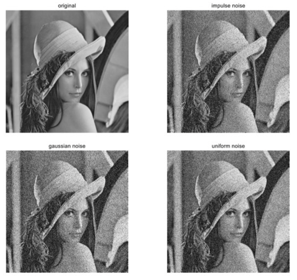
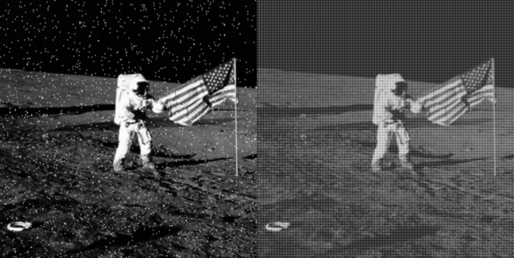
📍 예시_1
- 왼쪽 이미지의 경우 점과 같은 형체들이 이미지 전반에 걸쳐 노이즈처럼 분포
- 오른쪽 이미지의 경우 줄무늬와 같은 패턴의 노이즈가 이미지 전반에 걸쳐 분포
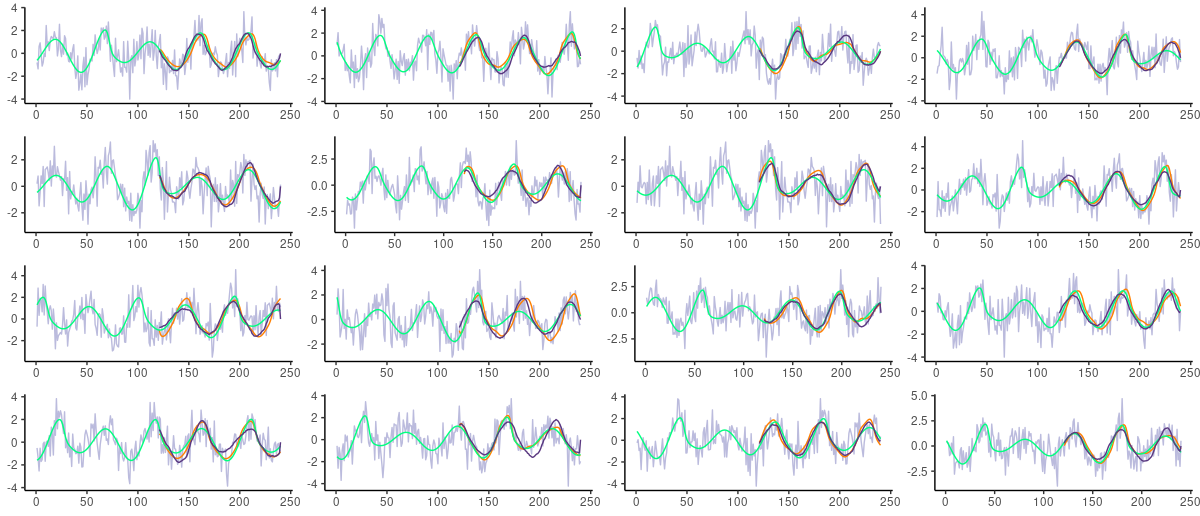
🔊 Noise in Time Series / Voice / Signal Data
👉 시계열/음성/신호에서의 Noise는 일반적으로 White Noise 또는 Gausian Noise로 발생
📄 Noise in Text Data
👉 일반적으로 철자 오류, 약어, 비표준단어, 반복, 구두점 누락, 대소문자 정보누락, 의성어 등의 원인에 의해 발생하는 Noise
👉 자동 음성인식, 광학 문자 인식, 기계 번역, web scraping 등으로 수집한 데이터에 Noise가 다수 존재
👉 자연어 처리의 성능을 저하시키는 요인
✏️ Denoising 이란?
👉 데이터의 Noise를 저감하여 모형이 더 좋은 성능을 보일 수 있도록 하는 전처리 과정
👉 Denoising 기법은 기본적으로 평활화(smoothing, 구간평균), 구간화(binning, 구간집계), 필터링(Filtering, 주파성분 저감) 기법을 사용
📅 정형 데이터의 디노이징
📖 평활화 (Smoothing)
👉 Noise로 인해 거칠게 분포된 데이터를 매끄럽게 만드는 기법
👉 Noise를 제거하기 위해 데이터 추세(Trend)에 벗어나는 값들을 변환하는 기법
👉 일반적으로 신호처리에서 많이 사용되나, 데이터 분석에서도 광범위하게 사용
👉 대표적으로 구간화(Binning)과 군집화(Clustering) 방법이 있음
1) 구간화 (Binning)
👉 정렬된 데이터 값들을 몇 개의 구간(bin)으로 분할하여 대표값으로 대체
(1) 동일 간격 (Equal-Distance) 구간화
👉 동일 간격으로 구간 설정
👉 정상 데이터가 한쪽으로 편중될 수 있으며 outlier에 의힌 영향을 많이 받음
👉 한쪽으로 몰려있는 데이터들은 모두 동일한 구간에 포함되기 때문에 왜도를 갖는 데이터(Skewed Data)를 다룰 수 없음
💻 코드 예시
import pandas as pd
import numpy as np

salary = pd.Series([4300, 8370, 1750, 3830, 1840, 4220, 3020, 2290, 4740, 4600,
                    2860, 3400, 4800, 4470, 2440, 4530, 4850, 4850, 4760, 4500,
                    4640, 3000, 1880, 4880, 2240, 4750, 2750, 2810, 3100, 4290,
                    1540, 2870, 1780, 4670, 4150, 2010, 3580, 1610, 2930, 4300,
                    2740, 1680, 3490, 4350, 1680, 6420, 8740, 8980, 9080, 3990,
                    4960, 3700, 9600, 9330, 5600, 4100, 1770, 8280, 3120, 1950,
                    4210, 2020, 3820, 3170, 6330, 2570, 6940, 8610, 5060, 6370,
                    9080, 3760, 8060, 2500, 4660, 1770, 9220, 3380, 2490, 3450,
                    1960, 7210, 5810, 9450, 8910, 3470, 7350, 8410, 7520, 9610,
                    5150, 2630, 5610, 2750, 7050, 3350, 9450, 7140, 4170, 3090])
#1 동일 간격으로 구간화 pd.cut()
df_salary = salary.sort_values()
cut_salary = pd.cut(df_salary, bins=5) # 구간을 몇 개로 나눌 것인지 입력하는 방법
cut_salary# result
30 (1531.93, 3154.0]
37 (1531.93, 3154.0]
44 (1531.93, 3154.0]
41 (1531.93, 3154.0]
2 (1531.93, 3154.0]
...
53 (7996.0, 9610.0]
83 (7996.0, 9610.0]
96 (7996.0, 9610.0]
52 (7996.0, 9610.0]
89 (7996.0, 9610.0]
Length: 100, dtype: category
Categories (5, interval[float64, right]): [(1531.93, 3154.0] < (3154.0, 4768.0] < (4768.0, 6382.0] < (6382.0, 7996.0] < (7996.0, 9610.0]]#2 동일 간격으로 구간화 pd.cut()
df_salary = salary.sort_values()
bins = [0, 2000, 4000, 6000, 8000, 10000] # 구간을 직접 지정하는 방법
cut_salary = pd.cut(df_salary, bins=bins)
cut_salary# result
30 (0, 2000]
37 (0, 2000]
44 (0, 2000]
41 (0, 2000]
2 (0, 2000]
...
53 (8000, 10000]
83 (8000, 10000]
96 (8000, 10000]
52 (8000, 10000]
89 (8000, 10000]
Length: 100, dtype: category
Categories (5, interval[int64, right]): [(0, 2000] < (2000, 4000] < (4000, 6000] < (6000, 8000] < (8000, 10000]](2) 동일 빈도 (Equal-Frequency) 구간화
- 동일한 개수의 데이터를 가지는 구간으로 구간 설정
💻 코드 예시
#3 동일 구간 수로 구간화 pd.qcut()
df_salary = salary.sort_values()
qcut_salary = pd.qcut(df_salary, q=5)
qcut_salary
# result
30 (1539.999, 2618.0]
37 (1539.999, 2618.0]
44 (1539.999, 2618.0]
41 (1539.999, 2618.0]
2 (1539.999, 2618.0]
...
53 (7068.0, 9610.0]
83 (7068.0, 9610.0]
96 (7068.0, 9610.0]
52 (7068.0, 9610.0]
89 (7068.0, 9610.0]
Length: 100, dtype: category
Categories (5, interval[float64, right]): [(1539.999, 2618.0] < (2618.0, 3544.0] < (3544.0, 4648.0] < (4648.0, 7068.0] < (7068.0, 9610.0]]df_qcut = pd.DataFrame(qcut_salary)
df_qcut.value_counts()# result
(1539.999, 2618.0] 20
(2618.0, 3544.0] 20
(3544.0, 4648.0] 20
(4648.0, 7068.0] 20
(7068.0, 9610.0] 20
Name: count, dtype: int64💻 구간 분할 후 대표값 대체 과정 코드 예시
import pandas as pd
import numpy as np
import matplotlib.pyplot as plt

df = pd.DataFrame({'uniform' : np.sort(np.random.uniform(0,10,10)),
                   'normal' : np.sort(np.random.normal(5,1,10)),
                   'gamma' : np.sort(np.random.gamma(2, size=10))})

col = 'uniform'
num_bins = 5

df_binned = pd.DataFrame()
df_binned[col] = df[col].sort_values()

df_binned['eq_dist_auto'] = pd.cut(df_binned[col], num_bins)
df_binned['eq_dist_fixed'] = pd.cut(df_binned[col], bins=[0,2,4,6,8,10])
df_binned['eq_freq_auto'] = pd.qcut(df_binned[col], num_bins)

cols = ['uniform','normal','gamma']

df_ew = df.copy()
for col in cols :
    df_ew[col+'_eq_dist'] = pd.cut(df_ew[col], 3) # 구간으로 나누기
    means = df_ew.groupby(col+'_eq_dist')[col].mean() # 구간의 평균값 계산
    df_ew.replace({col+'_eq_dist' : means}, inplace=True) # 평균값으로 대체

df_ef = df.copy()
for col in cols :
    df_ef[col+'_eq_freq'] = pd.cut(df_ef[col], 3) # 구간으로 나누기
    means = df_ef.groupby(col+'_eq_freq')[col].mean() # 구간의 평균값 계산
    df_ef.replace({col+'_eq_freq' : means}, inplace=True) # 평균값으로 대체

fig, axes = plt.subplots(1, 2, figsize=(10,5))
df_ew.astype(float).plot(ax=axes[0])
df_ef.astype(float).plot(ax=axes[1])
plt.show()
# result 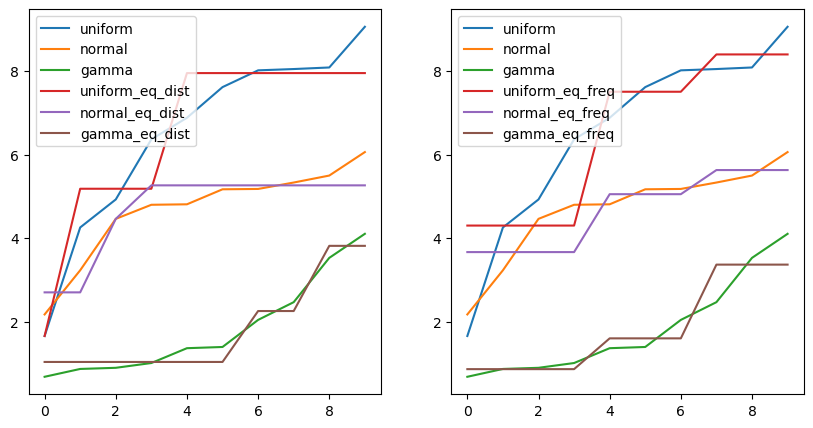
2) 군집화 (Clustering)
👉 유사한 값들을 하나의 군집으로 처리하여 중심점(centroid)을 대표값으로 대체
💻 코드 예시
from sklearn.preprocessing import KBinsDiscretizer

#1 동일한 간격으로 구간화 (Uniform)
ed_binner = KBinsDiscretizer(n_bins=3, encode='ordinal', strategy='uniform', subsample=None)
df_ed = ed_binner.fit_transform(df)

#2 동일한 빈도 수로 구간화 (quantile)
ef_binner = KBinsDiscretizer(n_bins=3, encode='ordinal', strategy='quantile', subsample=None)
df_ef = ef_binner.fit_transform(df)

#3 K-Means Clustering algorithm을 이용한 구간화 (kmeans)
km_binner = KBinsDiscretizer(n_bins=3, encode='ordinal', strategy='kmeans', subsample=None)
df_km = km_binner.fit_transform(df)

df_ed = pd.DataFrame(df_ed, columns=df.columns+'_eq_dist')
df_ef = pd.DataFrame(df_ef, columns=df.columns+'_eq_freq')
df_km = pd.DataFrame(df_km, columns=df.columns+'km')
df_bin = pd.concat([df, df_ed, df_ef, df_km], axis=1)

for bin_col in df_bin.columns :
    col = bin_col.split('_')[0]
    means = df_bin.groupby(by=bin_col)[col].mean()
    df_bin.replace({bin_col : means}, inplace=True)

fig, axes = plt.subplots(1, 3, figsize=(15,5))
pd.concat([df_bin.iloc[:,:3], df_bin.iloc[:,3:6]], axis=1).astype(float).plot(ax=axes[0])
pd.concat([df_bin.iloc[:,:3], df_bin.iloc[:,6:9]], axis=1).astype(float).plot(ax=axes[1])
pd.concat([df_bin.iloc[:,:3], df_bin.iloc[:,9:]], axis=1).astype(float).plot(ax=axes[2])
plt.show()
# result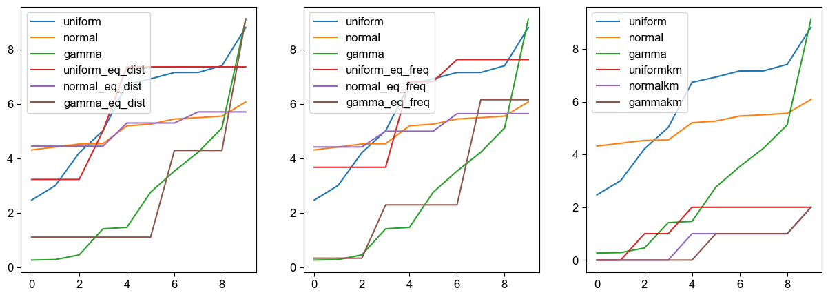
🙏 Reference
https://swrush.tistory.com/595
https://blog.naver.com/PostView.naver?blogId=laonple&logNo=220811027599
https://vincmazet.github.io/bip/restoration/denoising.html