[ML] Ensemble Learning and Random Forests

shihyunlim·2024년 11월 11일

Machine Learning

목록 보기

20/20

1) 앙상블 정의

앙상블: 일련의 예측기(한 개 아님!)
앙상블 학습: 일련의 예측기로부터 예측을 수집하여 더 나은 예측을 하는 것
앙상블 메소드: 앙상블 학습 알고리즘

2) 투표 기반 분류기

2-1) hard voting

hard voting(직접 투표): 여러 분류기의 예측을 집계하여, 가장 많이 나온 예측을 최종 예측으로 함(다수결 표)

각 분류기가 랜덤 추측보다 조금 높은 성능을 내는 weak learner일지라도 약한 학습기를 충분히 다양하게 모은 앙상블을 만든다면, 높은 정확도를 내는 strong learner가 될 수 있음(by law of large numbers)
모든 분류기는 완벽하게 독립적이고 오차에 상관관계가 없어야 정확한 예측을 할 수 있음
동일한 데이터에, 같은 분류기를 사용하면 같은 종류의 오차를 만들기 쉽기 때문에 잘못된 클래스가 다수일 수 있음. 그러므로 서로 다른 알고리즘으로 학습시키는 것이 서로 다른 오차를 만들 가능성이 높으므로, 앙상블에 각기 다른 분류기를 사용하는 것이 앙상블 성능에 좋을 수 있음

voting_clf = VotingClassifier(
	estimators=[
    	('lr', LogisticRegression(random_state=42)),
        ('rf', RandomForestClassifier(random_state=42)),
        ('svc', SVC(random_state=42))
    ]
)
voting_clf.fit(X_train, y_train)

VotingClassifier는 모든 추정기를 복제하여 복제된 추정기를 훈련함
- estimators 속성: 원본 추정기가 저장되는 곳
- estimators_: 훈련된 복제본
- named_estimators나 named_estimators: 리스트 대신 딕셔너리를 전달하는 경우
- predict로 예측하고 score를 통해 성능(점수)을 확인할 수 있음

2-2) soft voting

soft voting(간접 투표): predict_proba() 메소드와 같이 분류기의 확률을 예측할 수 있다면, 개별 분류기의 예측을 평균 내어 확률이 가장 높은 클래스를 예측하는 방법

확률이 높은 곳에 비중을 두므로, hard voting보다 성능이 높음
투표 기반 분류기의 voting 매개변수를 soft로 바꾸면 됨

voting_clf.voting = "soft"

# SVC는 클래스 확률을 기본적으로 제공하지 않으므로 따로 지정해줘야 함
voting_clf.named_estimators["svc"].probability = True

3) Bagging과 Pasting

앞에서 서로 다른 알고리즘을 사용한 앙상블을 만드는 것이 서로 다른 오차를 내기 때문에 더 나은 성능을 보일 수 있다고 했음. 이번에는 같은 알고리즘을 사용하는 대신 훈련 세트의 subset을 랜덤으로 구성하여 분류기를 서로 다르게 학습시키는 방법을 사용한다고 함. (완전히 동일한 데이터가 아니라 훈련 세트에서 subset을 나눠서 훈련하는 거라 괜찮은 건가?)

bagging: bootstrap aggregating의 줄임말. 훈련 세트에서 중복을 허용하여 샘플링하는 방식
pasting: 중복을 허용하지 않고 샘플링하는 방식

분류의 경우는 통계적 최빈값(hard voting과 동일)을, 회귀에서는 평균을 계산함
개별 예측기는 원본 훈련 세트로 훈련시킨 것보다 편향되어 있지만 집계 함수를 통과하면 편향과 분산이 모두 감소함. 일반적으로 앙상블은 원본 데이터셋을 하나의 예측기로 훈련시킬 때보다 편향은 비슷하지만 분산은 감소함
CPU 코어나 서버에서 병렬로 학습시킬 수 있음(확장성)
분류는 BaggingClassifier, 회귀는 BaggingRegressor로!
- pasting의 경우 bootstrap=False로 지정해야 함
- n_jobs: CPU 코어 수 지정, -1은 모든 코어를 사용한다는 것

bag_clf = BaggingClassifier(DecisionTreeClassifier(), n_estimators=500, max_samples=100, n_jobs=-1, random_state=42)
bag_clf.fit(X_train, y_train)

배깅을 사용하면 어떤 샘플은 여러 번 샘플링될 수 있지만, 또 다른 샘플은 사용되지 않을 수 있음. 평균적으로 63% 정도만 샘플링되고 나머지 37%는 샘플링되지 않음. 이를 "OOB(Out-of-bag) 샘플"이라고 함
검증 셋 대신에 OOB를 사용하여 모델을 평가할 수 있음. oob_score=True로 지정하기

bag_clf = BaggingClassifier(DecisionTreeClassifier(), n_estimators=500, oob_score=True, n_jobs=-1, random_state=42)

# 점수 확인
bag_clf.oob_score_

# 기반 예측기가 predict_proba()를 가지는 경우. 아래와 같이 클래스 별 확률 확인 가능
bag_clf.oob_decision_function[:3]

4) Random patches method와 Random subspaces method

BaggingClassifier는 앞에서 샘플을 조정하는 max_samples, bootstrap 말고도 특성을 샘플링하는 max_features, bootstrap_features가 있음! 특성 샘플링은 더 다양한 예측기를 만들며 편향을 늘리는 대신 분산을 줄임

Random patches method: 훈련 특성과 샘플을 모두 샘플링
Random subspaces method: 훈련 샘플은 모두 사용(bootstrap=False, max_samples=1.0), 특성만 샘플링bootstrap_features=True, max_features은 1.0보다 작게)

5) Random Forest

일반적으로 bagging 방법을 적용한 결정 트리의 앙상블
일반적으로 max_sample를 훈련 세트의 크기로 지정
노드를 분할할 때 최선의 특성을 찾는 것이 아닌 랜덤으로 특성 후보를 선택하여 그 중에서 최적의 특성을 찾는 방법을 택함. 무작위성이 더 주입됨
- 전체 특성 수가 n일 때 $\sqrt{n}$ 개의 특성을 선택
- 편향이 커지지만 분산을 낮추어 결과적으로 더 좋은 모델 만듦

rnd_clf = RandomForestClassifier(n_estimators=500, max_leaf_nodes=16, n_jobs=-1, random_state=42)
rnd_clf.fit(X_train, y_train)
y_pred_rf = rnd_clf.predict(X_test)

5-1) extremly randomized tree ensemble (-> extra tree)

극단적으로 랜덤한 트리의 랜덤 포레스트
편향이 증가하는 대신 분산이 낮아짐
일반 랜덤 포레스트는 모든 노드에서 특성마다 최고의 임곗값을 구하느라 시간이 많이 소요되지만 엑스트라 트리의 경우 무작위 분할 후 최적값을 선택하기 때문에 빠름(최적의 분할을 계산하는 것이 아님)
참고: https://velog.io/@nata0919/Extra-Trees-%EC%A0%95%EB%A6%AC, https://takethat.tistory.com/38
ExtraTreesClassifier를 사용

5-2) 특성의 상대적 중요도 측정

노드의 어떤 특성이 불순도를 평균적으로 얼마나 감소시키는지 확인
구체적으로, 노드에 사용된 특성별로 (현재 노드의 샘플 비율 x 불순도) - (왼쪽 자식 노드의 샘플 비율 x 불순도) - (오른쪽 자식의 샘플 비율 x 불순도)를 계산하고 특성 중요도의 합이 1이 되도록 전체 합으로 나누어 정규화함
- 샘플 비율: 트리 전체 샘플 수에 대한 비율
랜덤 포레스트의 특성 중요도는 각 결정 트리의 특성 중요도를 모두 합하여 트리 수로 나눈 것

6) Boosting

약한 학습기를 여러 개 연결하여 강한 학습기를 만드는 것. 앞의 모델을 보완하며 순차적으로 예측기를 학습시키는 것

6-1) AdaBoost(Adaptive boosting)

'에이다부스트'라고 읽는대.. 처음 알았네
이전 모델이 과소적합했던(잘못 분류되었던) 훈련 샘플의 가중치를 더 높이는 방법
모든 예측기가 순차적으로 학습을 마치면 앞의 배깅이나 페이스팅과 같은 방식으로 최종 예측을 함. 그런데 에이다부스트에서는 모델을 훈련한 후 가중치를 부여하기 때문에 최종 예측을 할 때 훈련 세트의 정확도에 따라 예측기마다 다른 가중치를 부여해야 함!
순차적인 학습을 하기 때문에 병렬 불가. 확장성 높지 않음

수식 메모

각 샘플의 가중치 = $w^{(i)}$
$w^{(i)}=\frac{1}{m}$ 으로 초기화

j번째 예측기 학습 후 가중치가 적용된 오차율 = $r_j$

r_j = \frac{\sum_{\substack{i=1 \\ \hat{y}_j^{(i)} \neq y^{(i)}}}^{m} w^{(i)}}{\sum_{i=1}^{m} w^{(i)}}

-> $\hat{y}_j^{(i)} \neq y^{(i)}$ : i번째 샘플에 대한 예측( $\hat{y}_j^{(i)}$ )과 실제값( $y^{(i)}$ )이 다른 경우
-> 이 경우 가중치의 합을 전체 가중치의 합으로 나누므로 오차율이라고 함!

예측기의 가중치 = $\alpha_j$

\alpha_j = \eta\log\frac{1-r_j}{r_j}

-> $\eta$ : 학습률, 기본값=1
-> 예측이 정확하면 $\alpha$ 는 증가하며 양수임. 랜덤 예측인 경우 $\alpha$ 는 0에 가까움. 예측이 이보다 더 나쁘면 $\alpha$ 는 음수

가중치 $w^{(i)}$ 업데이트 규칙

w^{(i)} \leftarrow \begin{cases} w^{(i)} & \text{if }\hat{y}_j^{(i)} = y^{(i)} \\ w^{(i)} \exp(\alpha_j) & \text{if } \hat{y}_j^{(i)} \neq y^{(i)} \end{cases} \quad \text{where } i = 1, 2, \dots, m

-> 예측기 학습 및 업데이트 과정은 전체 예측기 수 또는 지정된 예측기의 수만큼 반복 후 종료됨

Adaboost의 최종 예측

\hat{y}(\mathbf{x}) = \arg\max_{k} \sum_{\substack{j=1 \\ \hat{y}_j(\mathbf{x}) = k}}^{N} \alpha_j

-> $k$ : 클래스
-> 모든 예측기( $j$ )의 예측을 계산하고, 예측기 가중치 $\alpha_j$ 를 더하여 최종 예측 결과인 $\hat{y}(\mathbf{x})$ 를 만듦. arg max k로 나와 있으므로 가중치 합이 가장 큰 클래스의 인자(argument)가 $\hat{y}(\mathbf{x})$ 이 되는 것을 알 수 있음!

ada_clf = AdaBoostClassifier(
	DecisionTreeClassifier(max_depth=1), n_estimators=30, learning_rate=0.5, random_state=42)
ada_clf.fit(X_train, y_train)

6-2) Gradient Boosting

each new model is trained to minimize the loss function of the previous model using gradient descent
in contrast to AdaBoost, the weights of the training instances are not tweaked, instead, each predictor is trained using the residual errors of the predecessor as labels

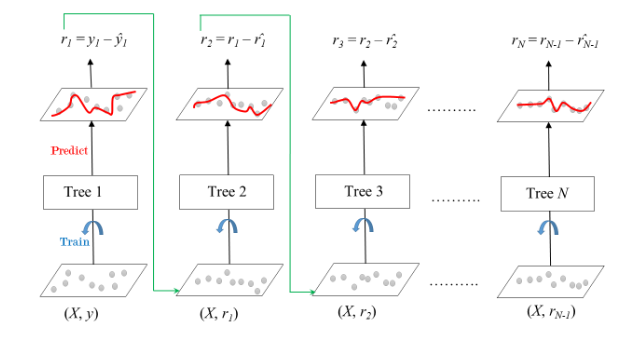
As shown above, Tree1 is trained using the feature matrix X and the labels y. The predictions labeled y1(hat) are used to determine the training set residual errors r1. Tree2 is then trained using the feature matrix X and the residual errors r1 of Tree1 as labels. The predicted results r1(hat) are then used to determine the residual r2. The process is repeated until all the M trees forming the ensemble are trained.

There is an important parameter used in this technique known as Shrinkage. Shrinkage refers to the fact that the prediction of each tree in the ensemble is shrunk after it is multiplied by the learning rate(eta) which ranges between 0 to 1.

There is a trade-off between eta and the number of estimators, decreasing learning rate needs to be compensated with increasing estimators in order to reach certain model performance.

After all trees being trained, predictions can be made. Each tree predicts a label and the final prediction is given by the formula:

y(pred) = y1 + (eta *  r1) + (eta * r2) + ....... + (eta * rN)

출처: https://www.geeksforgeeks.org/ml-gradient-boosting/

gbrt_best = GradientBoostingRegressor(
	max_depth=2, learning_rate=0.05, n_estimators=500, n_iter_no_change=10, random_state=42)

n_iters_no_change=10: 마지막 10개의 트리가 도움이 되지 않는 경우 훈련을 자동으로 중지
subsample=0.25: 각 트리는 랜덤으로 선택된 25%의 훈련 샘플로 학습 -> stochastic GD

(Histogram-based gradient boosting 내용 생략)

7) Stacking(stacked generalization)

The idea is that you can attack a learning problem with different types of models which are capable to learn some part of the problem, but not the whole space of the problem.

So, you can build multiple different learners and you use them to build an intermediate prediction, one prediction for each learned model. Then you add a new model which learns from the intermediate predictions the same target.

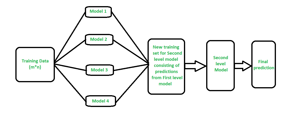
How stacking works?

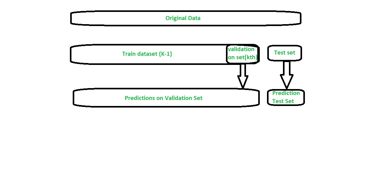
We split the training data into K-folds just like K-fold cross-validation.
A base model is fitted on the K-1 parts and predictions are made for Kth part.
We do for each part of the training data.
The base model is then fitted on the whole train data set to calculate its performance on the test set.
We repeat the last 3 steps for other base models.
Predictions from the train set are used as features for the second level model.
Second level model is used to make a prediction on the test set.

출처: https://www.geeksforgeeks.org/stacking-in-machine-learning/

stacking_clf = StackingClassifier(
	estimators=[
    ('lr': LogisisticRegression(random_state=42)),
    ('rf': RandomForestClassifier(random_state=42)),
    ('svc': SVC(probability=True, (random_state=42))
	],
	final_estimator=RandomForestClassifier(random_state=42), cv=5 # 교차 검증 폴드 수
)

shihyunlim

이전 포스트