06.10 전집중 호흡 복습|전처리&시각화 2회차|오오. 이 또한 귀도 반 로섬 선생님의 혜안이겠지요

이틀 연속 엉덩이 왕.

항상 그렇듯 library를 먼저 import 하자

import pandas as pd
import numpy as np
import seaborn as sns
import matplotlib.pyplot as plt

오늘도 타이타닉을 쓸 거다

url = "https://raw.githubusercontent.com/datasciencedojo/datasets/master/titanic.csv"

titanic = pd.read_csv(url)

먼저 대충 크기를 보자 .shape

titanic.shape
#(891, 12) < row, column

전체적인 통계치를 먼저 보자 .describe()

titanic.describe()

분위 수를 나눠서 더 자세히 보자.describe(percentiles=[.1,.25,.75,.9,.95])

detailed_stats = titanic.describe(percentiles=[.1,.25,.75,.9,.95])
detailed_stats.round(2)

더 많은 범주형 데이터를 보려면.describe(include='all')

titanic.describe(include='all')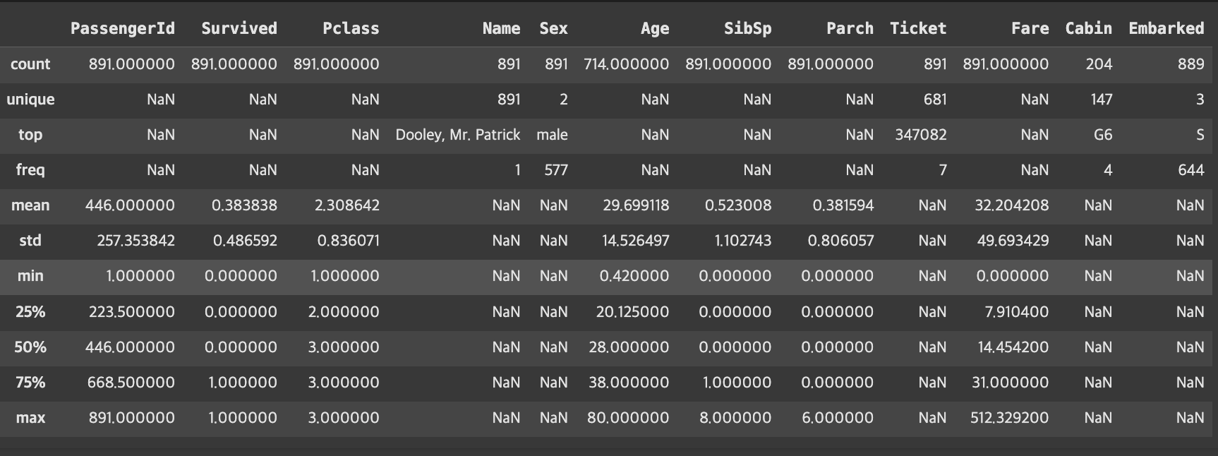

항목	설명
count	각 열에서 결측치(NaN)를 제외한 값의 개수
unique	고유 값의 개수 (범주형 변수에서 유용)
top	가장 많이 등장한 값 (최빈값)
freq	최빈값의 빈도 수
mean	평균값
std	표준편차 (standard deviation), 값들이 평균에서 얼마나 떨어져 있는지를 나타냄
min	최솟값
25% (Q1)	제1사분위수: 전체 데이터 중 25%가 이 값보다 작거나 같음
50% (Q2)	중앙값(Median): 전체 데이터 중 50%가 이 값보다 작거나 같음. 이상치에 덜 민감함
75% (Q3)	제3사분위수: 전체 데이터 중 75%가 이 값보다 작거나 같음
max	최댓값

---

📍범주형 데이터의 빈도를 ARABOZA

범주형?| 값이 몇 개의 카테고리로 정해진 데이터

Value_counts() method로 카테고리별 갯수, 정규화 값(normalize=true)을 구해보자

sex_counts = titanic['Sex'].value_counts()
sex_ratios = titanic['Sex'].value_counts(normalize=True)
기본이 normalize=false로 설정 되어 있는 거기 때문에 false 집어 넣으면 그냥 갯수만 나옴.
normalize=True는 "정규화=해라"라는 뜻임

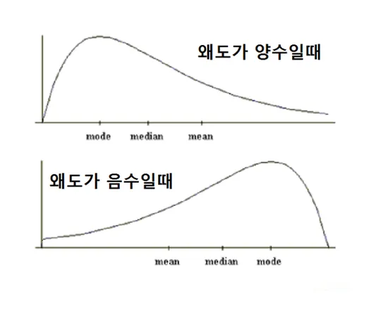
📍분포의 형태 파악하기! 데이터의 치우침<왜도>, 데이터의 중앙 밀집 <첨도>

왜도[Skewness]

• 데이터의 분포가 치우친 정도를 계산하는 방법
• 정규분포처럼 분포가 좌우대칭을 이룰수록 왜도값은 0으로 수렴
  
  왜도가 양수면...| 몇몇 큰 데이터가 평균을 끌어올렸다는 것
  왜도가 음수면...| 몇몇 작은 데이터가 펭균을 끌어내렸다는 것

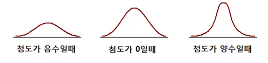
첨도[Kurtosis]

• 데이터의 중앙 집중도를 보여주는 척도
  첨도가 음수면...| 완만함. 데이터가 전체적으로 튀지 않고 고르다는 것. 극단값이 거의 없다는 것.
  첨도가 0에 가까우면....| 정규분포 정도의 뾰족함. 보통 신체 등급 따위에서 많이 나오는 것.
  첨도가 양수면...| 데이터가 튄다는 것. 극단 값이 존재하기 때문에 위험하다는 것. (outliar)

---

describe data frame에서 값을 뽑아 보자

age_stats = titanic['Age'].describe()
mean_age= age_stats['mean'] #mean
median_age=age_stats['50%'] #중앙값 50%
print(mean_age)
print(median_age)

📍분포의 치우침 판단은 중앙값과 평균값으로
평균>중앙값: 오른쪽으로 치우침
평균<중위수: 왼쪽으로 치우짐

if mean_age > median_age:
    print("→ 평균 > 중위수: 오른쪽으로 치우친 분포")
    print("  (고령자 일부가 평균을 끌어올림)")
else:
    print("→ 평균 ≤ 중위수: 왼쪽으로 치우친 분포")

왜도와 첨도, 메써드로도 구할 수 있어요!| skew(), kurtosis()

# 왜도와 첨도로 분포 특성 정량화
age_data = titanic['Age'].dropna()
#결측치 버려서 오류 버리기
skewness = age_data.skew()
#왜도skewness계산
kurtosis = age_data.kurtosis()
#첨도kurtosis계산
print(f"왜도(Skewness): {skewness:.3f}")
print(f"첨도(Kurtosis): {kurtosis:.3f}")
#.3f는 소숫점 셋째 자리까지 반올림 round는 원본이 바뀌어버림. 3f는 보이는 형태만 바꿈.

• 왜도 > 0: 오른쪽 꼬리가 긴 분포 (양의 왜도)
• 왜도 < 0: 왼쪽 꼬리가 긴 분포 (음의 왜도)
• 첨도 > 3: 정규분포보다 뾰족한 분포
• 첨도 < 3: 정규분포보다 평평한 분포

---

📍생존률과 탑승 좌석, 관련 있나요? 상관관계 메서드 .Corr() [Correlation Matrix]

# 주요 숫자형 변수들의 상관관계 numeric 숫자 cols열의 correlation상관관계
numeric_cols = ['Survived', 'Pclass', 'Age', 'SibSp', 'Parch', 'Fare']
correlation_matrix = titanic[numeric_cols].corr()
print(correlation_matrix.round(3))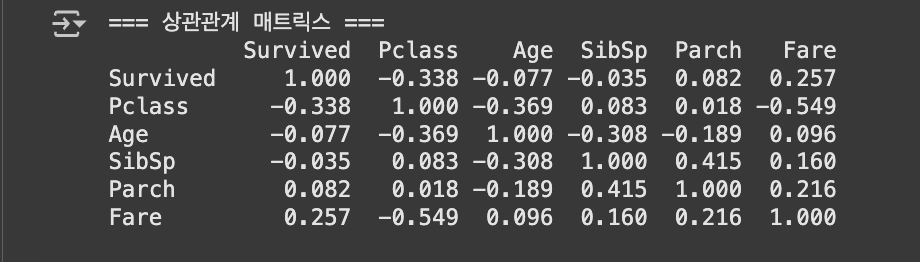

• 0.7 이상: 매우 강한 상관관계
• 0.3~0.7: 강한 상관관계
• 0.1~0.3: 중간 상관관계
• 0.1 미만: 약한 상관관계

절댓값으로 survived와 관련이 깊은 상관관계 순위 매기기

survival_corr = correlation_matrix['Survived'].drop('Survived')

survived는 자기자신이니까 버리기. 이러면 시리즈가 할당 되겠지?

survival_corr_sorted = survival_corr.reindex(survival_corr.abs()
.sort_values(ascending=False).index)

.reindex()| 인덱스 순서를 바꾸겠다.
abs()| 절댓값 치환.
sort_values(ascending=False)| 나열/descending으로.
.index()| 인덱스 형태로 변환

print("=== 생존과의 상관관계 (강한 순) ===")
for var, corr in survival_corr_sorted.items():
    strength = "강함" if abs(corr) > 0.3 else "중간" if abs(corr) > 0.1 else "약함"
    direction = "양의" if corr > 0 else "음의"
    print(f"{var:8s}: {corr:6.3f} ({direction} {strength})")
    

#{var:8s} → 변수 이름 8칸 맞춤
#{corr:6.3f} → 소수점 3자리까지, 전체 6칸 공간 확보

결과값 대조하면서 읽어보기

# 주요 상관관계 해석
pclass_corr = survival_corr['Pclass']
fare_corr = survival_corr['Fare']

print(f"객실등급과 생존: {pclass_corr:.3f} (음의 상관관계)")
print("→ 등급 숫자가 작을수록(1등석) 생존율이 높음")
print(f"운임과 생존: {fare_corr:.3f} (양의 상관관계)")
print("→ 운임이 높을수록 생존율이 높음")
print("→ 경제적 여건이 생존에 영향을 미쳤을 가능성")

import seaborn as sns
import matplotlib.pyplot as plt

# 히트맵 시각화
plt.figure(figsize=(8, 6))  # 그림 크기 설정
sns.heatmap(correlation_matrix, 
            annot=True,        # 셀 안에 숫자 표시
            fmt=".2f",         # 소수점 둘째 자리까지
            cmap="coolwarm",   # 색상 테마
            vmin=-1, vmax=1)   # 색상의 범위 고정

plt.title("Titanic Numeric Features Correlation Heatmap")
plt.tight_layout()
plt.show()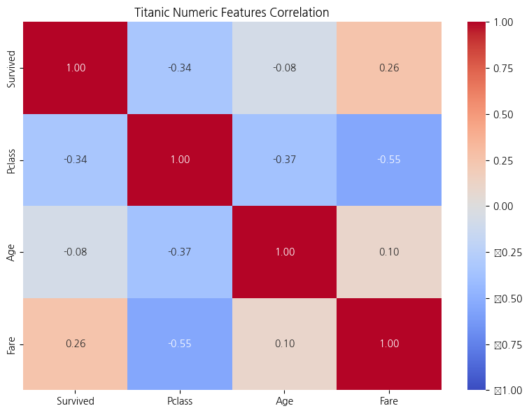

---

결측치 처리 마스터 하기

결측치란?
데이터 값이 없거나 누락된 상태. 처리하지 않으면 왜곡이나 오류 발생.

---

기본 결측치 확인

print("=== 컬럼별 결측치 개수 ===")
missing_counts = titanic.isnull().sum()
print(missing_counts)

count는 왜 안 써요? > count쓰면 Notnull도 같이 새게 됨. isnull이 기본적으로 False값 즉 1이기 때문에 sum으로 새는 것임.

결측치 비율 계산 (더 중요!)

print("=== 컬럼별 결측치 비율 ===")
missing_ratios = (titanic.isnull().sum() / len(titanic) * 100).round(2)
missing_summary = pd.DataFrame({
    '결측치_개수': missing_counts,
    '결측치_비율(%)': missing_ratios
})

결측치가 있는 컬럼만 표시

missing_summary = missing_summary[missing_summary['결측치_개수'] > 0]
print(missing_summary.sort_values('결측치_비율(%)', ascending=False))

결측치 제거(신중하라!)

데이터 크기 먼저 확인해 보자

titanic.shape

결측치 존재행 삭제(dropna())

titanic_dropped_missings = titanic.dropna()
titanic_dropped_missings.shape #row column
len(titanic)-len(titanic_dropped_missings #결측행 값
1- len(titanic_dropped_missings)/len(titanic)*100:.3f)#데이터 손실률

언제 사용해야 할까?

• 결측치 비율이 5% 미만일 때
• 결측치 패턴이 완전 무작위일 때
• 충분한 데이터가 남을 때

⚠️ 주의사항:

위 결과에서 보듯이 너무 많은 데이터가 손실될 수 있습니다.

결측치 있는 컬럼만 삭제

list는 차집합이 안되니까 집합함수인 set으로 묶어서 차집합 계산
axis는 축이라는 의미 axis=0은 row axis=1은 column

titanic_dropped_cols = titanic.dropna(axis=1) #컬럼을 기준으로 빈 칼럼 삭제
print(f"결측치 컬럼 삭제 후: {titanic_dropped_cols.shape}")
print(f"삭제된 컬럼: {set(titanic.columns) - set(titanic_dropped_cols.columns)}")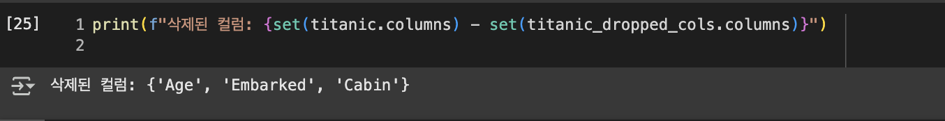

컬럼 삭제는 언제?

• 결측치 비율이 50% 이상인 컬럼
• 분석에 중요하지 않은 컬럼
• 다른 변수로 대체 가능한 정보를 담은 컬럼
• subset(dropna, fillna) 옵션의 전략적 활용 모든 컬럼이 아닌 분석에 필수적인 컬럼 의 결측치만 제거

특정 컬럼의 결측치만 있는 행 삭제

\n = 줄바꿈

titanic_age_dropped = titanic.dropna(subset=['Age'])
print(f"\nAge 결측치만 삭제 후: {titanic_age_dropped.shape}")
print(f"Age 결측치로 삭제된 행: {len(titanic) - len(titanic_age_dropped)}개")

📌 결측치 대체 전략 선택 가이드

• 평균값: 정규분포에 가까운 연속형 변수
• 중위수: 이상치가 많거나 치우친 분포
• 최빈값: 범주형 변수
• 특정값: 비즈니스 로직상 의미가 있는 값
• 예측값: 다른 변수들로 예측한 값

---

값을 대체 해보자

숫자형 값의 대체

필드 복사

titanic_filled = titanic.copy()

describe()로 기본 통계 확인

print("=== Age 기본 통계 ===")
age_stats = titanic['Age'].describe()
print(f"평균: {age_stats['mean']:.1f}세")
print(f"중위수: {age_stats['50%']:.1f}세") 
print(f"표준편차: {age_stats['std']:.1f}")
print(f"결측치: {titanic['Age'].isnull().sum()}개")

평균값으로 대체

age_mean=titanic_filled['Age'].mean()
titanic_filled['Age_mean_filled']=titanic_filled['Age'].fillna(age_mean).astype(int)
titanic_filled

print(f"\n평균값({age_mean:.1f}세)으로 대체 완료")
print(f"대체 후 결측치: {titanic_filled['Age_mean_filled'].isnull().sum()}개")

평균값 대체
장점: 전체 평균에 영향 주지 않음
단점: 변수의 다양성 감소. 극값(outliar)이 있을 때 불안정

---

중위수로 대체 (이상치에 덜 민감)

age_median = titanic_filled['Age'].median()
titanic_filled['Age_median_filled'] = titanic_filled['Age'].fillna(age_median)

print(f"중위수({age_median:.1f}세)으로 대체 완료")

데이터에 극값이 많을 떄 이상적

대체 방법별 분포 비교

print("\n=== 대체 방법별 통계 비교 ===")
comparison = pd.DataFrame({
    '원본': titanic['Age'].describe(),
    '평균대체': titanic_filled['Age_mean_filled'].describe(),
    '중위수대체': titanic_filled['Age_median_filled'].describe()
}).round(2)
print(comparison)

범주형 값의 대체 embarked(승선위치) 예시

결측치 개수 보기

#분포도 먼저 보기
print("=== Embarked 결측치 분석 ===")
embarked_counts = titanic['Embarked'].value_counts()
print("Embarked 분포:")
#빈 칸 확인하기
print(embarked_counts)
print(f"결측치: {titanic['Embarked'].isnull().sum()}개")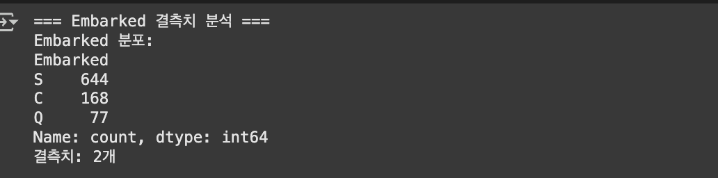

본격 대치 소동. 최빈값(.mode())으로 대체 해보자

embarked_mode = titanic['Embarked'].mode()[0]  
# mode()는 Series를 반환하므로 [0]  최빈값이 여러 개일 수 있으니까!
embarked_mode
#최빈값 S가 nan값에 할당 됨

titanic_filled['Embarked_filled'] = titanic_filled['Embarked'].fillna(embarked_mode)