References:
이번 포스팅에서는 3D Computer vision에서 필수적인 개념인 camera calibration의 개념에 대해서 알아보자.
Introduction
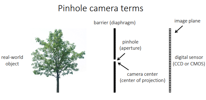
3D 공간상에서 어떤 장면을 카메라로 찍고 있다고 하자. 이때 3D 공간 상의 장면은 카메라 렌즈를 통해 2D 이미지로 projection된다.
Computer vision에서 가장 중요한 문제 중 하나는 이렇게 카메라로 찍은 2D image로부터 3D scene을 복원해내는 것이다.
즉, 2D image의 각 pixel point가 현실의 3D 공간인 world coordinate frame의 정확히 어떤 점에 위치하게 되는지 알아내야 한다.
이렇게 2D image로부터 3D scene을 복원하기 위해서는 아래의 2가지가 필요하다.
-
External parameters of the camera
World coordinate frame에 대한 카메라의 position과 orientation에 대한 정보
-
Internal parameters of the camera
카메라가 3D에서 projection한 point를 어떻게 image plane으로 mapping하는 지에 대한 정보 (e.g., focal length)
그리고 camera의 external / internal parameter를 결정하는 작업을 Camera Calibration이라고 한다.
Camera calibration에 대해 아래의 순서대로 차근차근 공부해보자.
1) Camera Model / Forward Imaging Model
2) Camera Calibration
3) Intrinsic and Extrinsic Matrices
Camera Model / Forward Imaging Model
3D point를 image의 pixel로 projection해주는 역할을 수행하는 camera model을 먼저 정해야 한다. 이때 camera model은 linear model로 정하고, 이는 보통 pinhole camera라고도 불린다.
이러한 Linear Camera Model은 하나의 matrix 형태로 표현될 수 있는데, 이를 projection matrix라고 부른다.
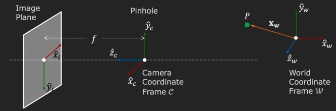
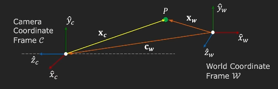
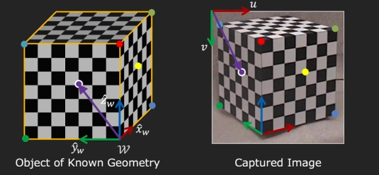
위의 그림처럼 world coordinate frame w에 어떤 point P가 위치했다고 하자.
이 world coordinate frame에 카메라가 있다고 하자. 그러면 camera도 camera만의 coordinate C를 가진다. 이때 camera coordinate frame의 Z축은 카메라의 optical axis와 align되어있다.
** optical axis
카메라 lens 중심과 image sensor 중심을 잇는 가상의 선으로, pinhole camera의 경우 pinhole을 지나는 선이다.
그리고 여기서 f는 effective focal length로 lens와 image sensor사이의 거리를 의미한다.
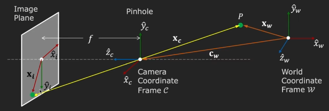
만약에 우리가 world coordinate frame에 대한 camera coordinate frame의 상대적인 position과 orientation을 알고 있다면 (주황색 선 cw로 표현), 우리는 point P로부터 그것의 image plane의 projection xi를 구해낼 수 있게 된다 (노란색 선으로 표현).
이러한 mapping 자체를 forward imaging model이라고 한다.
Perspective Projection
먼저 Perspective Projection부터 알아보자. 이는 camera coordinate에 있는 좌표를 image coordinate로 projection시키는 과정이다.
이때, camera coordinate 값을 z값으로 나누어 normalized plane으로 옮기고 (camera coordinate에서 정의된 point들을 z=1인 plane위로 옮겨놓는 작업), focal length값에 따라 image plane 상에서 scaling하게 된다.
fxi=zcxcandfyi=zcyc
그러므로,
xi=fzcxcandyi=fzcyc
그런데, 여기서 조금 더 고려해줘야할 사항이 있다.
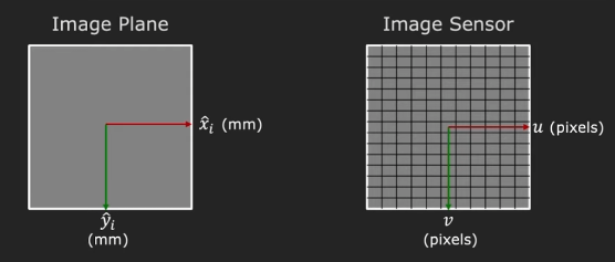
우리가 image plane의 xi,yi를 알고 있다고 해도, 이는 camera coordinate frame에서 정의되었던 단위인, mm와 같은 단위의 값일 것이다.
하지만 실제로 우리는 이미지 센서를 통해 이미지를 보기 때문에, 이미지 센서의 pixel 입장에서 생각해야한다. 즉, image coordinate를 mm에서 pixel로 mapping 시켜줘야한다.
u=mxfzcxcandv=myfzcyc
여기서 mx,my를 pixel density (pixels/mm)라고 한다.
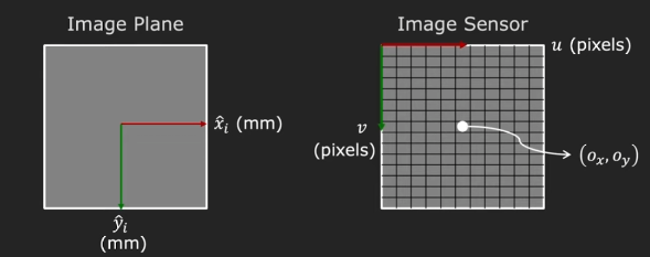
두번째로는 optical axis가 image plane과 만나는 지점인 principle point의 위치를 정확히 알지 못한다는 점이다. 그래서 이것에 대한 보정을 추가로 해주어야 한다.
추가적으로 보통 이미지 sensor의 origin을 top-left corner로 사용하기 때문에, principle point가 (ox,oy)라고 하면, 최종적으로 image sensor의 좌표는 아래와 같이 구할 수 있다.
u=mxfzcxc+oxandv=myfzcyc+oy
Focal length를 pixel로 표현하여 x,y 방향에 대해 표현하면, 아래와 같이 쓸 수 있다.
u=fxzcxc+oxandv=fyzcyc+oy
여기서, 우리가 모르는 값인 (fx,fy,ox,oy)를 camera의 Intrinsic parameters라고 하며, 이는 camera 자체의 internal geometry을 나타낸다.
Homogeneous coordinate
Perspective projection의 문제는 바로 식이 Non-linear하다는 것이다.
u=fxzcxc+oxandv=fyzcyc+oy
이 문제를 해결하기 위해 homogenous representation을 도입하는데, 이는 기존의 cartesian coordinate에 임의로 추가적인 dimension을 추가하여 normalized plane에서 표현하는 방식으로, geometric transformation을 더욱 간단한 식으로 만들어준다.
조금 더 직관적으로 생각해보자.
Perspective projection은 y=Ax+b로 표현되는 affine transformation 으로, linear transformation과 다르게 translation이 포함되는데, 이 projection / transformation matrix는 이마저도 y=Ax의 형태로 한꺼번에 표현하고자 하는 것이 homogenous representation이다.
그래서 linear transformation matrix에 transformation matrix가 추가된 형태를 띄게 되고, N차원 벡터를 표현할 때, N+1차원 벡터가 사용된다.
벡터 차원을 추가할 때는, 마지막 차원에 단순히 w을 더한 형태로 표현되며, w값에 따라 homogenous representation은 무한히 존재한다. 즉, k라는 scaling에 대해서 아래 좌표는 모두 같은 좌표를 표현하게 된다.
⎣⎢⎡kukvkw⎦⎥⎤≡⎣⎢⎡uvw⎦⎥⎤
쉽게 이야기 해서 2D point u=(u,v)를 3D point u~=(u~,v~,w~) (w~=0)로 표현하는 것이고, 원래의 u,v를 구할 때는 3D point에서 끝 자리가 1이 되도록 w~를 나누어서 구한다.
u≡⎣⎢⎡uv1⎦⎥⎤≡⎣⎢⎡w~uw~vw~⎦⎥⎤≡⎣⎢⎡u~v~w~⎦⎥⎤=u~
3D point에서 4D point로의 homogenous representation도 똑같다.
x≡⎣⎢⎢⎢⎡xyz1⎦⎥⎥⎥⎤≡⎣⎢⎢⎢⎡w~xw~yw~zw~⎦⎥⎥⎥⎤≡⎣⎢⎢⎢⎡x~y~z~w~⎦⎥⎥⎥⎤=x~
Intrinsic Matrix
그러면 다시 Perspective Projection으로 돌아가보자.
u=fxzcxc+oxandv=fyzcyc+oy
여기서 (u,v)에 homogenous coordinate를 적용하면 분모의 zc를 옮겨서 표현할 수 있고, 나아가 하나의 matrix를 이용하여 더욱 간단하게 표현할 수 있다.
⎣⎢⎡uv1⎦⎥⎤≡⎣⎢⎡u~v~w~⎦⎥⎤≡⎣⎢⎡zcuzcvzc⎦⎥⎤=⎣⎢⎡fxxc+zcoxfyyc+zcoyzc⎦⎥⎤=⎣⎢⎡fx000fy0oxoy1000⎦⎥⎤⎣⎢⎢⎢⎡xcyczc1⎦⎥⎥⎥⎤
마지막 matrix 곱을 보면 왼쪽 3×4 matrix는 모든 camera internal paramter를 포함하고, 오른쪽 4×1는 3차원 camera coordinate의 homogeneous representation이다.
이렇게 우리는 perspective projection의 linear model을 유도해냈다. 그리고 이 internal parameter를 포함한 3×4 matrix를 Intrinsic Matrix라고 한다.
Intrinsic matrix를 조금 더 분해해보면 앞의 3×3 matrix를 calibration matrix라고 하며, upper right triangular matrix 형태이다.
K=⎣⎢⎡fx000fy0oxoy1⎦⎥⎤
정리하자면 3D camera coordinate frame에서 2D pixel coordinate로의 prespective projection은 아래와 같이 표현할 수 있다.
u~=[K∣0]x~c=Mintrinsicx~c
Extrinsic Parameters
이제 perspective projection을 잘 정의했으니, 이제 world coordinate에서 camera coordinate로의 3D-to-3D mapping을 잘 정의해보자.
이는 camera coordinate frame의 position과 orientation을 이용하면 된다.
World coordinate frame w에서 camera의 Position cw와 Orientation R을 camera의 Extrinsic Parameter라고 한다.
Rotation은 3×3 matrix로 표현되는데, 이 matrix의 각 row는 world coordinate에서 camera coordinate의 각 basis의 direction로도 해석할 수 있다.
⎣⎢⎡r11r21r31r12r22r32r13r23r33⎦⎥⎤→Row1:x^cinw→Row2:y^cinw→Row3:z^cinw
그러므로 중요한 점은 이 Rotation matrix가 Orthonormal하다는 것이다.
* Orthonormal이란?
두 벡터 u와 v에 대해,
1) dot(u,v)=uTv=0
2) uTu=vTv=1
어떤 square matrix의 row나 column vector가 orthonormal하다면,
1) R−1=RT
2) RTR=RRT=I
이제는 Extrinsic parameter가 주어졌다면, camera frame으로부터의 P의 위치 (노란색 벡터)를 camera coordinate frame에서 계산할 수 있다.
xc=R(xw−cw)
xw와 cw의 벡터 뺄셈을 통해 world coordiante frame에서 xc를 구할 수 있고, 여기에 rotation matrix를 곱하면 camera coordinate frame에서의 xc, 즉 P의 위치를 구할 수 있다.
이를 조금 풀어서 나눠쓰면 translation vector t를 나눠줄 수 있고,
xc=R(xw−cw)=Rxw−Rcw=Rxw+t
t=−Rcw
Matrix형태로 쓰면 아래와 같이 표현할 수 있다.
xc=⎣⎢⎡xcyczc⎦⎥⎤=⎣⎢⎡r11r21r31r12r22r32r13r23r33⎦⎥⎤⎣⎢⎡xwywzw⎦⎥⎤+⎣⎢⎡txtytz⎦⎥⎤
위 식을 하나의 4×4 matrix로 합쳐 표현하기 위해 다시한번 homogenous coordinate를 도입하면,
x~c=⎣⎢⎢⎢⎡xcyczc1⎦⎥⎥⎥⎤=⎣⎢⎢⎢⎡r11r21r310r12r22r320r13r23r330txtytz1⎦⎥⎥⎥⎤⎣⎢⎢⎢⎡xwywzw1⎦⎥⎥⎥⎤
바로 이 matrix가 camera의 Extrinsic Matrix라고 하며, World to Camera coordinate transformation은 아래와 같이 표현할 수 있다.
x~c=[R3×303×3t1]x~w=Mextrinsicx~w
Projection Matrix
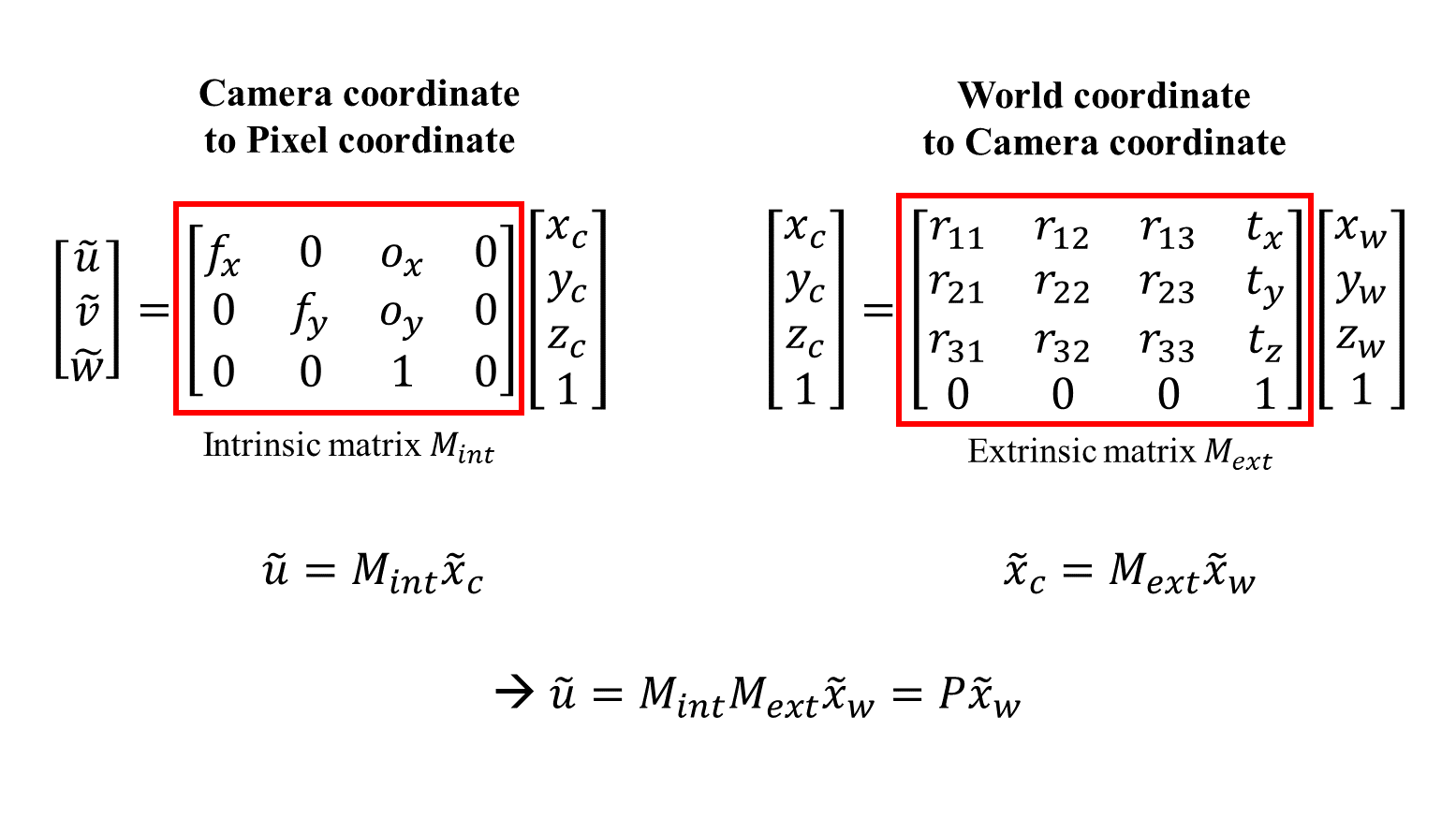
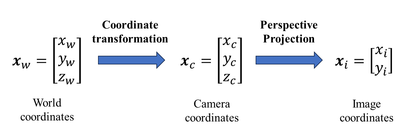
정리하자면 우리는 camera의 extrinsic matrix를 통해 world coordinate에서 camera coordinate로 mapping하고, intrinsic matrix를 통해 camera coordinate에서 pixel coordniate로 mapping한다.
이 연산은 두 matrix를 연속적으로 곱해서 가능하고, 이를 하나의 3×4 의 projection matrix P를 이용할 수 있다.
Camera를 calibration하기 위해서는 projection matrix만 찾으면 된다. Projection matrix를 구했다면 3D space의 어떤 점도 image위로 projection 시킬 수 있다.
Camera Calibration
Projection Matrix를 이해했으므로, 이제 우리는 Camera Calibration을 할 수 있다.
Camera Calibration은 projection matrix를 추정하는 것이다.
Camera calibration을 위해서는 어떤 known geometry상에 있는 object를 찍은 image를 이용한다.
먼저, geometry를 알고 있는 (모든 point의 location 정보가 있는..) 어떤 3D 공간에 world coordinate를 정의한다.
World coordinate는 기호대로 어떤 corner로 잡으면 된다. 그러면 그 coordinate를 기반으로 모든 점의 좌표값이 정해지게 된다.
그리고, 이를 카메라로 찍은 하나의 이미지를 생각하자. 그리고 world coordinate의 임의의 point (보라색 점)를 잡으면, 그 좌표를 알 수 있고, image coordinate의 픽셀 값도 찾을 수 있다.
예를 들어,
xw=⎣⎢⎡xwywzw⎦⎥⎤=⎣⎢⎡034⎦⎥⎤u=[uv]=[56115]
이렇게 3D scene과 2D image 사이에 corresponding point를 많이 찾으면, 각각의 point i에 대해 아래의 식이 성립한다.
⎣⎢⎡u(i)v(i)1⎦⎥⎤≡⎣⎢⎡p11p21p31p12p22p32p13p23p33p14p24p34⎦⎥⎤⎣⎢⎢⎢⎢⎡xw(i)yw(i)zw(i)1⎦⎥⎥⎥⎥⎤
위 matrix를 linear equation으로 풀어서 쓰면 아래와 같이 쓸 수 있는데,
u(i)=p31xw(i)+p32yw(i)+p33zw(i)+p34p11xw(i)+p12yw(i)+p13zw(i)+p14
v(i)=p31xw(i)+p32yw(i)+p33zw(i)+p34p21xw(i)+p22yw(i)+p23zw(i)+p24
분모를 양변에 곱하고 식을 넘기면 우리가 하는 모든 값과 우리가 모르는 projection matrix component (12개)의 matrix multiplication으로 표현할 수 있게 된다.
A(known)⋅⎣⎢⎢⎢⎢⎢⎢⎢⎢⎢⎡p11p12p13...p32p33p34⎦⎥⎥⎥⎥⎥⎥⎥⎥⎥⎤=⎣⎢⎢⎢⎢⎢⎢⎢⎢⎢⎡000...000⎦⎥⎥⎥⎥⎥⎥⎥⎥⎥⎤
여기서 projection matrix의 재밌는 성질이 하나 나오는데, 바로 projection matrix가 homogenous coordinate 상에서 작동한다는 것이다.
즉, projection matrix를 scaling해도 같은 homogenous pixel coordinate를 도출하게 된다는 것이다.
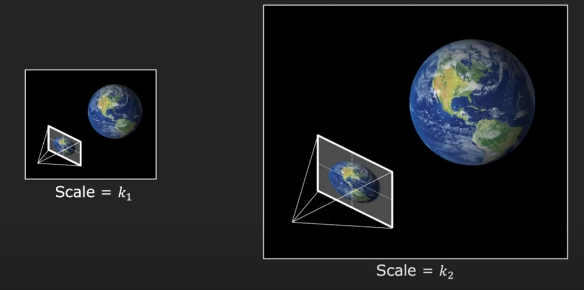
Projection matrix를 scale한다는 것은 내가 대상으로 하는 world와 camera의 size를 동시에 scaling한다는 것으로, 얻어지는 이미지는 변하지 않는다.
또한 이 말은 projection matrix의 scale을 임의로 정해줄 수 있다는 것으로도 볼 수 있다.
최종적으로는 위에서 구한 식에서 Ap를 최대한 0에 가깝게하고, p의 scale을 계산하기 쉽게 잡아서 P를 구하면 된다. (Constrained Least Squares Problem)
minp∣∣Ap∣∣2s.t.∣∣p2∣∣=1
이렇게 projection matrix를 estimation하는 것을 calibration이라고 한다.
지금까지 Calibration method를 통해, projection matrix를 얻는 방법을 알아보았는데, calibration은 intrinsic / extrinsic matrix를 구하지않고 직접 projection matrix를 구하므로, 이제 projection matrix로부터 intrinsic matrix와 extrinsic matrix를 다시 decompose하는 방법을 알아보자.
Projection matrix를 intrinsic matrix와 extrinsic matrix로 나누어 쓰면 아래와 같다.
p=⎣⎢⎡p11p21p31p12p22p32p13p23p33p14p24p34⎦⎥⎤=⎣⎢⎡fx000fy0oxoy1000⎦⎥⎤⎣⎢⎢⎢⎡r11r21r310r12r22r320r13r23r330txtytz1⎦⎥⎥⎥⎤
이때, 행렬곱을 생각해보면 projection matrix의 앞 3×3 matrix는 사실 위에서 알아본 calibration matrix와 rotation matrix의 곱인 것을 알 수 있다.
⎣⎢⎡p11p21p31p12p22p32p13p23p33⎦⎥⎤=⎣⎢⎡fx000fy0oxoy1⎦⎥⎤⎣⎢⎡r11r21r31r12r22r32r13r23r33⎦⎥⎤=KR
그런데 우리는 calibration matrix는 Upper-right triangular matrix이고, rotation marix는 Orthonomal matrix라는 사실을 알고 있기 때문에, 선형대수의 QR factorization을 통해 K와 R을 decompose할 수 있게 된다.
마지막으로 translation을 생각해보면, 이는 projection matrix의 마지막 열에서부터 쉽게 구해낼 수 있다.
⎣⎢⎡p14p24p34⎦⎥⎤=⎣⎢⎡fx000fy0oxoy1⎦⎥⎤⎣⎢⎡txtytz⎦⎥⎤=Kt
방금 위에서 K를 구했으므로, 이것의 역행렬을 이용하여 t를 계산할 수 있다.
t=K−1⎣⎢⎡p14p24p34⎦⎥⎤
Discussion
이번 포스팅에서는 camera calibration의 개념에 대해서 알아보면서, Coordinate system과 linear camera model, 그리고 camera의 intrinsic/extrinsic matrix에 대해 알아보았다.
3D computer vision 논문을 읽으면서 꼭 필요한 개념이라고 생각이 되서 공부하다가 좋은 강의 영상을 찾아서 이를 토대로 정리해보았다.