YOLOv3 head 이해

Reference
https://github.com/ultralytics/yolov3/blob/master/models/yolo.py
https://wikidocs.net/163607

YOLO HEAD detail

Detection network는 head에서 output을 처리하는 부분이 매번 헷갈리는 것 같다.

YOLOv3의 head는 v4에서도 동일하게 사용되니, 조금 더 명확하게 이해해보도록 하자.

먼저, YOLOv3은 feature extractor의 feature map으로부터 1x1 convolution을 통해 output을 도출한다.

즉 feature map의 각 위치 (cell)에 대해 각각 output이 정의된다는 말이고, 이 output은 feature map과 같은 $H \times W$를 가지며, depth 방향으로, 각 cell마다 ($B \times (1 +4 +C)$)개의 값을 가진다.

그리고 각 cell은 각자의 위치에서, 그 cell이 responsible한 gt bounding box를 예측하게 된다. 그리고 responsible하다는 기준은 bounding box의 중심점이 그 cell 안에 떨어질 때로 정했다.

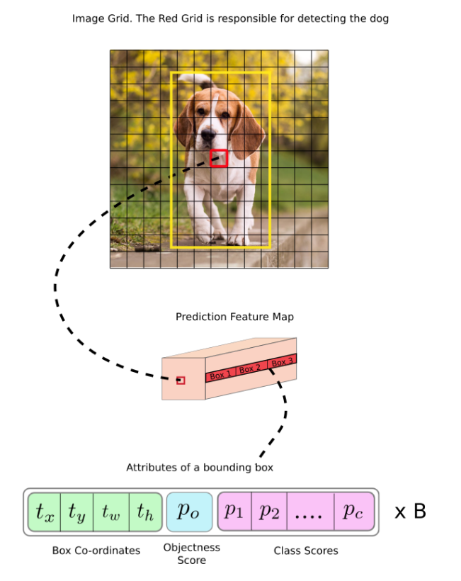
예를 들어 위 그림의 경우, 귀여운 강아지 bbox의 중심점이 속해있는 $(6,6)$ cell 혹은 grid가 강아지를 detection하는 데 responsible하다.

그럼 이제 이 cell에서 prediction을 했다고 하자. 다음으로는 이 prediction을 ground truth와 비교하여 loss를 구하고 네트워크를 학습시켜야한다.

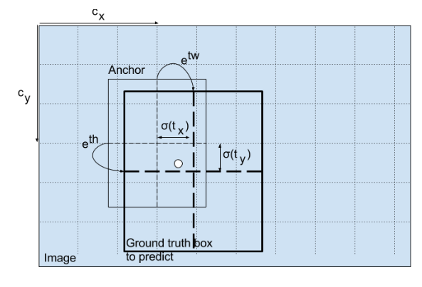
하지만 1 혹은 0의 값을 예측해야하는 classification과 다르게, bounding box의 경우 center point 이외에도 width와 height를 예측해야하는데, 직접적으로 이러한 값들을 loss calculation에 사용하게 되면, 안정적으로 학습을 하기가 어렵다.

그래서 도입된 개념이 바로 anchor box이다. Anchor box는 GT box를 예측하기 위한 매개체이자 pre-defined bounding box로, 각 cell 별로 몇 개의 서로 다른 ratio를 가지는 box를 미리 정의해 두고, 네트워크는 이 anchor의 offset을 예측해서 gt box와 최대한 match시키려고 한다.

하나의 object를 나타내는 bounding box는 하나인게 자연스러우므로, GT box와 IOU가 가장 큰 anchor가 다시 그 object를 detecting하는데 responsible한 anchor가 된다.

즉, 실제 GT box의 center point를 포함하는 cell이 해당 box에 responsible하고, 이 cell의 prediction값들은 '이 cell에 대해 정의된 anchor box들 중 GT box와 가장 IOU 값이 큰 anchor'의 offset이다.

최종적으로 YOLOv3는 3개의 서로 다른 scale feature로부터 output을 내고, 각 prediction feature의 cell 하나 당 3개의 bounding box를 predict하므로,

YOLOv3는 한 이미지당 $(3 \times (scale _1\times scale_1+scale _2\times scale_2+scale _3\times scale_3))$개의 bounding box prediction을 생성한다.

Code review

YOLOv3의 코드를 통해서도 실제로 detection가 어떻게 작동하는지 알아보자.

출처: https://github.com/ultralytics/yolov3/blob/master/models/yolo.py

class Detect(nn.Module):
    # YOLOv3 Detect head for detection models
    stride = None  # strides computed during build
    dynamic = False  # force grid reconstruction
    export = False  # export mode

    def __init__(self, nc=80, anchors=(), ch=(), inplace=True):  # detection layer
        super().__init__()
        self.nc = nc  # number of classes
        self.no = nc + 5  # number of outputs per anchor
        self.nl = len(anchors)  # number of detection layers
        self.na = len(anchors[0]) // 2  # number of anchors
        self.grid = [torch.empty(0) for _ in range(self.nl)]  # init grid
        self.anchor_grid = [torch.empty(0) for _ in range(self.nl)]  # init anchor grid
        self.register_buffer("anchors", torch.tensor(anchors).float().view(self.nl, -1, 2))  # shape(nl,na,2)
        self.m = nn.ModuleList(nn.Conv2d(x, self.no * self.na, 1) for x in ch)  # output conv
        self.inplace = inplace  # use inplace ops (e.g. slice assignment)

    def forward(self, x):
        z = []  # inference output
        for i in range(self.nl):
            x[i] = self.m[i](x[i])  # conv
            bs, _, ny, nx = x[i].shape  # x(bs,255,20,20) to x(bs,3,20,20,85)
            x[i] = x[i].view(bs, self.na, self.no, ny, nx).permute(0, 1, 3, 4, 2).contiguous()

            if not self.training:  # inference
                if self.dynamic or self.grid[i].shape[2:4] != x[i].shape[2:4]:
                    self.grid[i], self.anchor_grid[i] = self._make_grid(nx, ny, i)

                if isinstance(self, Segment):  # (boxes + masks)
                    xy, wh, conf, mask = x[i].split((2, 2, self.nc + 1, self.no - self.nc - 5), 4)
                    xy = (xy.sigmoid() * 2 + self.grid[i]) * self.stride[i]  # xy
                    wh = (wh.sigmoid() * 2) ** 2 * self.anchor_grid[i]  # wh
                    y = torch.cat((xy, wh, conf.sigmoid(), mask), 4)
                else:  # Detect (boxes only)
                    xy, wh, conf = x[i].sigmoid().split((2, 2, self.nc + 1), 4)
                    xy = (xy * 2 + self.grid[i]) * self.stride[i]  # xy
                    wh = (wh * 2) ** 2 * self.anchor_grid[i]  # wh
                    y = torch.cat((xy, wh, conf), 4)
                z.append(y.view(bs, self.na * nx * ny, self.no))

        return x if self.training else (torch.cat(z, 1),) if self.export else (torch.cat(z, 1), x)

    def _make_grid(self, nx=20, ny=20, i=0, torch_1_10=check_version(torch.__version__, "1.10.0")):
        d = self.anchors[i].device
        t = self.anchors[i].dtype
        shape = 1, self.na, ny, nx, 2  # grid shape
        y, x = torch.arange(ny, device=d, dtype=t), torch.arange(nx, device=d, dtype=t)
        yv, xv = torch.meshgrid(y, x, indexing="ij") if torch_1_10 else torch.meshgrid(y, x)  # torch>=0.7 compatibility
        grid = torch.stack((xv, yv), 2).expand(shape) - 0.5  # add grid offset, i.e. y = 2.0 * x - 0.5
        anchor_grid = (self.anchors[i] * self.stride[i]).view((1, self.na, 1, 1, 2)).expand(shape)
        return grid, anchor_grid

Detect class instance variables

self.nc = nc  # number of classes
self.no = nc + 5  # number of outputs per anchor
self.nl = len(anchors)  # number of detection layers
self.na = len(anchors[0]) // 2  # number of anchors
self.grid = [torch.empty(0) for _ in range(self.nl)]  # init grid
self.anchor_grid = [torch.empty(0) for _ in range(self.nl)]  # init anchor grid
self.register_buffer("anchors", torch.tensor(anchors).float().view(self.nl, -1, 2))  # shape(nl,na,2)
self.m = nn.ModuleList(nn.Conv2d(x, self.no * self.na, 1) for x in ch)  # output conv
self.inplace = inplace  # use inplace ops (e.g. slice assignment)

• self.no : 각 anchor의 output 갯수 -> 4개의 bounding box 정보 (x, y, width, height)와 1개의 objectness score, nc개의 per class prediction (YOLOv3 논문에서는 80개)
• self.nl : detection layer의 갯수 (YOLOv3 논문에서는 서로 다른 scale의 layer 3개 이용)
• self.na : 각 scale에서 anchor의 갯수 (=각 cell의 anchor 갯수)
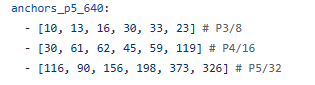
  pre-defined anchor는 아래와 같이 정의되어있으며, 각 line의 각 scale을 의미하고, 한 line는 3개의 anchor에 대한 size pair 정보를 담고있다.
  --> [width,height,width,height,width,height]

• self.grid & self.anchor_grid : inference 시, bounding box coordinate를 계산하기 위함
• self.m : 위에서 설명한 $1\times 1$ conv layer의 list이며, backbone으로부터 얻어진 feature의 channel을 desired output 갯수인self.no * self.na로 늘려주기 위함

Forward function 1) Training

def forward(self, x):
    z = []  # inference output
    for i in range(self.nl):
        x[i] = self.m[i](x[i])  # conv
        bs, _, ny, nx = x[i].shape  # x(bs,255,20,20) to x(bs,3,20,20,85)
        x[i] = x[i].view(bs, self.na, self.no, ny, nx).permute(0, 1, 3, 4, 2).contiguous()

return x if self.training

• 서로 다른 scale의 feature에 대해, $1 \times 1$ conv를 수행
• 그러면 feature map의 각 grid cell에 대해 channel 방향으로 $3*(80+5)=255$개의 값을 만들어냄
• tensor를 reshape해서 anchor dimension을 따로 빼냄
  (batch_size, num_anchors, grid_height, grid_width, num_outputs)
• 최종 return 값은 각 scale에 대한 위 tensor의 list $x$

학습 시에는 이 x값을 그대로 return한다.

return된 prediction은 이후 간단한 processing을 거쳐 gt와 loss를 구하는데 사용된다.

Loss calculation

loss는 어떻게 계산되는지 알아보자.

class ComputeLoss:
    sort_obj_iou = False

    # Compute losses
    def __init__(self, model, autobalance=False):
        device = next(model.parameters()).device  # get model device
        h = model.hyp  # hyperparameters

        # Define criteria
        BCEcls = nn.BCEWithLogitsLoss(pos_weight=torch.tensor([h["cls_pw"]], device=device))
        BCEobj = nn.BCEWithLogitsLoss(pos_weight=torch.tensor([h["obj_pw"]], device=device))

        # Class label smoothing https://arxiv.org/pdf/1902.04103.pdf eqn 3
        self.cp, self.cn = smooth_BCE(eps=h.get("label_smoothing", 0.0))  # positive, negative BCE targets

        # Focal loss
        g = h["fl_gamma"]  # focal loss gamma
        if g > 0:
            BCEcls, BCEobj = FocalLoss(BCEcls, g), FocalLoss(BCEobj, g)

        m = de_parallel(model).model[-1]  # Detect() module
        self.balance = {3: [4.0, 1.0, 0.4]}.get(m.nl, [4.0, 1.0, 0.25, 0.06, 0.02])  # P3-P7
        self.ssi = list(m.stride).index(16) if autobalance else 0  # stride 16 index
        self.BCEcls, self.BCEobj, self.gr, self.hyp, self.autobalance = BCEcls, BCEobj, 1.0, h, autobalance
        self.na = m.na  # number of anchors
        self.nc = m.nc  # number of classes
        self.nl = m.nl  # number of layers
        self.anchors = m.anchors
        self.device = device

    def __call__(self, p, targets):  # predictions, targets
        lcls = torch.zeros(1, device=self.device)  # class loss
        lbox = torch.zeros(1, device=self.device)  # box loss
        lobj = torch.zeros(1, device=self.device)  # object loss
        tcls, tbox, indices, anchors = self.build_targets(p, targets)  # targets

        # Losses
        for i, pi in enumerate(p):  # layer index, layer predictions
            b, a, gj, gi = indices[i]  # image, anchor, gridy, gridx
            tobj = torch.zeros(pi.shape[:4], dtype=pi.dtype, device=self.device)  # target obj

            n = b.shape[0]  # number of targets
            if n:
                # pxy, pwh, _, pcls = pi[b, a, gj, gi].tensor_split((2, 4, 5), dim=1)  # faster, requires torch 1.8.0
                pxy, pwh, _, pcls = pi[b, a, gj, gi].split((2, 2, 1, self.nc), 1)  # target-subset of predictions

                # Regression
                pxy = pxy.sigmoid() * 2 - 0.5
                pwh = (pwh.sigmoid() * 2) ** 2 * anchors[i]
                pbox = torch.cat((pxy, pwh), 1)  # predicted box
                iou = bbox_iou(pbox, tbox[i], CIoU=True).squeeze()  # iou(prediction, target)
                lbox += (1.0 - iou).mean()  # iou loss

                # Objectness
                iou = iou.detach().clamp(0).type(tobj.dtype)
                if self.sort_obj_iou:
                    j = iou.argsort()
                    b, a, gj, gi, iou = b[j], a[j], gj[j], gi[j], iou[j]
                if self.gr < 1:
                    iou = (1.0 - self.gr) + self.gr * iou
                tobj[b, a, gj, gi] = iou  # iou ratio

                # Classification
                if self.nc > 1:  # cls loss (only if multiple classes)
                    t = torch.full_like(pcls, self.cn, device=self.device)  # targets
                    t[range(n), tcls[i]] = self.cp
                    lcls += self.BCEcls(pcls, t)  # BCE

                # Append targets to text file
                # with open('targets.txt', 'a') as file:
                #     [file.write('%11.5g ' * 4 % tuple(x) + '\n') for x in torch.cat((txy[i], twh[i]), 1)]

            obji = self.BCEobj(pi[..., 4], tobj)
            lobj += obji * self.balance[i]  # obj loss
            if self.autobalance:
                self.balance[i] = self.balance[i] * 0.9999 + 0.0001 / obji.detach().item()

        if self.autobalance:
            self.balance = [x / self.balance[self.ssi] for x in self.balance]
        lbox *= self.hyp["box"]
        lobj *= self.hyp["obj"]
        lcls *= self.hyp["cls"]
        bs = tobj.shape[0]  # batch size

        return (lbox + lobj + lcls) * bs, torch.cat((lbox, lobj, lcls)).detach()

    def build_targets(self, p, targets):
        # Build targets for compute_loss(), input targets(image,class,x,y,w,h)
        na, nt = self.na, targets.shape[0]  # number of anchors, targets
        tcls, tbox, indices, anch = [], [], [], []
        gain = torch.ones(7, device=self.device)  # normalized to gridspace gain
        ai = torch.arange(na, device=self.device).float().view(na, 1).repeat(1, nt)  # same as .repeat_interleave(nt)
        targets = torch.cat((targets.repeat(na, 1, 1), ai[..., None]), 2)  # append anchor indices

        g = 0.5  # bias
        off = (
            torch.tensor(
                [
                    [0, 0],
                    [1, 0],
                    [0, 1],
                    [-1, 0],
                    [0, -1],  # j,k,l,m
                    # [1, 1], [1, -1], [-1, 1], [-1, -1],  # jk,jm,lk,lm
                ],
                device=self.device,
            ).float()
            * g
        )  # offsets

        for i in range(self.nl):
            anchors, shape = self.anchors[i], p[i].shape
            gain[2:6] = torch.tensor(shape)[[3, 2, 3, 2]]  # xyxy gain

            # Match targets to anchors
            t = targets * gain  # shape(3,n,7)
            if nt:
                # Matches
                r = t[..., 4:6] / anchors[:, None]  # wh ratio
                j = torch.max(r, 1 / r).max(2)[0] < self.hyp["anchor_t"]  # compare
                # j = wh_iou(anchors, t[:, 4:6]) > model.hyp['iou_t']  # iou(3,n)=wh_iou(anchors(3,2), gwh(n,2))
                t = t[j]  # filter

                # Offsets
                gxy = t[:, 2:4]  # grid xy
                gxi = gain[[2, 3]] - gxy  # inverse
                j, k = ((gxy % 1 < g) & (gxy > 1)).T
                l, m = ((gxi % 1 < g) & (gxi > 1)).T
                j = torch.stack((torch.ones_like(j), j, k, l, m))
                t = t.repeat((5, 1, 1))[j]
                offsets = (torch.zeros_like(gxy)[None] + off[:, None])[j]
            else:
                t = targets[0]
                offsets = 0

            # Define
            bc, gxy, gwh, a = t.chunk(4, 1)  # (image, class), grid xy, grid wh, anchors
            a, (b, c) = a.long().view(-1), bc.long().T  # anchors, image, class
            gij = (gxy - offsets).long()
            gi, gj = gij.T  # grid indices

            # Append
            indices.append((b, a, gj.clamp_(0, shape[2] - 1), gi.clamp_(0, shape[3] - 1)))  # image, anchor, grid
            tbox.append(torch.cat((gxy - gij, gwh), 1))  # box
            anch.append(anchors[a])  # anchors
            tcls.append(c)  # class

        return tcls, tbox, indices, anch

코드가 너무 복잡하니까 __call__함수만 집중

1) Initialize loss

lcls = torch.zeros(1, device=self.device)  # Initialize class loss
lbox = torch.zeros(1, device=self.device)  # Initialize box loss (IoU loss)
lobj = torch.zeros(1, device=self.device)  # Initialize objectness loss
tcls, tbox, indices, anchors = self.build_targets(p, targets)  # Build targets

• self.build_targets 함수를 통해 raw target data를 알맞은 format으로 변환

2) Build target

na, nt = self.na, targets.shape[0]  # number of anchors, targets
tcls, tbox, indices, anch = [], [], [], []
gain = torch.ones(7, device=self.device)  # normalized to gridspace gain
ai = torch.arange(na, device=self.device).float().view(na, 1).repeat(1, nt)  # same as .repeat_interleave(nt)
targets = torch.cat((targets.repeat(na, 1, 1), ai[..., None]), 2)  # append anchor indices

• na는 cell별 anchor 갯수, nt는 target의 갯수 (batch안 gt box의 총 갯수)
• target은 [num of boxes, 6]의 shape을 가지며, 각 row는 (image index in a batch, class label, x,y,w,h)을 represent
• 각 target을 anchor 갯수만큼 복제 -> 이후에 각 anchor를 모든 target gt box와 비교하기 위함
• 추가로 ai를 통해 anchor의 indices를 하나의 dimension으로 추가 -> 최종 targets shape = (na, nt, 7)

g = 0.5  # bias
off = (
    torch.tensor(
    [
    [0, 0],
    [1, 0],
    [0, 1],
    [-1, 0],
    [0, -1],  # j,k,l,m
    # [1, 1], [1, -1], [-1, 1], [-1, -1],  # jk,jm,lk,lm
    ],
    device=self.device,
    ).float()
    * g
)  # offsets

• Bounding box의 center point를 조정하기 위한 변수 선언

for i in range(self.nl):
    anchors, shape = self.anchors[i], p[i].shape
    gain[2:6] = torch.tensor(shape)[[3, 2, 3, 2]]  # xyxy gain

    # Match targets to anchors
    t = targets * gain  # shape(3,n,7)

• 서로 다른 scale에 대해 iterate
• self.anchors는 $(nl,na,2)$ shape의 tensor -> anchors는 현재 scale의 anchor
• shape은 각 layer의 prediction의 shape = (batch_size, num_anchors, grid_height, grid_width, num_outputs)
• gain은 target의 좌표를 해당 scale feature map과 맞춰주기 위한 값으로, [1,1,scale_x,scale_y,scale_x,scale_y,1]의 값을 가진다.
• target에 gain을 곱해서 target의 좌표 부분을 scaling

    if nt:
        # Matches
        r = t[..., 4:6] / anchors[:, None]  # wh ratio
        j = torch.max(r, 1 / r).max(2)[0] < self.hyp["anchor_t"]  # compare
        # j = wh_iou(anchors, t[:, 4:6]) > model.hyp['iou_t']  # iou(3,n)=wh_iou(anchors(3,2), gwh(n,2))
        t = t[j]  # filter

        # Offsets
        gxy = t[:, 2:4]  # grid xy
        gxi = gain[[2, 3]] - gxy  # inverse
        j, k = ((gxy % 1 < g) & (gxy > 1)).T
        l, m = ((gxi % 1 < g) & (gxi > 1)).T
        j = torch.stack((torch.ones_like(j), j, k, l, m))
        t = t.repeat((5, 1, 1))[j]
        offsets = (torch.zeros_like(gxy)[None] + off[:, None])[j]
    else:
        t = targets[0]
        offsets = 0

• r은 t에서 width, height를 추출하여 anchor와 비교한 결과로, width/height ratio값을 가짐. shape = (na, nt, 2)
• j는 r이나 r의 역수에서도 width/height ratio중에 가장 높은 값을 의미하고, 이 값이 특정 hyperparameter보다 작아야한다. r이 1에 가까워야 j가 True이라는 것이고, 이말은 즉 gt를 가장 잘 표현하는 anchor를 찾는다는 것.
• 위에서 filtering한 target box에 대해 offset 계산 -> feature에서의 grid indices를 찾기 위함

# Define
    bc, gxy, gwh, a = t.chunk(4, 1)  # (image, class), grid xy, grid wh, anchors
    a, (b, c) = a.long().view(-1), bc.long().T  # anchors, image, class
    gij = (gxy - offsets).long()
    gi, gj = gij.T  # grid indices

    # Append
    indices.append((b, a, gj.clamp_(0, shape[2] - 1), gi.clamp_(0, shape[3] - 1)))  # image, anchor, grid
    tbox.append(torch.cat((gxy - gij, gwh), 1))  # box
    anch.append(anchors[a])  # anchors
    tcls.append(c)  # class

return tcls, tbox, indices, anch

• t.chunk(4,1) : t를 dim=1에서 4등분
  t -> [image idx, class | x, y | w, h | anchor idx]
• target에 대한 processing을 마친 뒤, 아래의 결과들을 return
  • target classes list
  • target bounding boxes list
  • batch indices, anchor indices, grid indices
  • anchor list (해당 indices의 anchor들)

3) Loss 계산

이제 잘 처리된 target을 가지고 network prediction과 loss를 계산할 수 있다.

# Losses
for i, pi in enumerate(p):  # layer index, layer predictions
    b, a, gj, gi = indices[i]  # image, anchor, gridy, gridx
    tobj = torch.zeros(pi.shape[:4], dtype=pi.dtype, device=self.device)  # target obj

    n = b.shape[0]  # number of targets
    if n:
        # pxy, pwh, _, pcls = pi[b, a, gj, gi].tensor_split((2, 4, 5), dim=1)  # faster, requires torch 1.8.0
        pxy, pwh, _, pcls = pi[b, a, gj, gi].split((2, 2, 1, self.nc), 1)  # target-subset of predictions
        
        # Regression
    	pxy = pxy.sigmoid() * 2 - 0.5
    	pwh = (pwh.sigmoid() * 2) ** 2 * anchors[i]
    	pbox = torch.cat((pxy, pwh), 1)  # predicted box
    	iou = bbox_iou(pbox, tbox[i], CIoU=True).squeeze()  # iou(prediction, target)
    	lbox += (1.0 - iou).mean()  # iou loss

    	# Objectness
    	iou = iou.detach().clamp(0).type(tobj.dtype)
    	if self.sort_obj_iou:
        	j = iou.argsort()
        	b, a, gj, gi, iou = b[j], a[j], gj[j], gi[j], iou[j]
    	if self.gr < 1:
        	iou = (1.0 - self.gr) + self.gr * iou
    	tobj[b, a, gj, gi] = iou  # iou ratio

    	# Classification
    	if self.nc > 1:  # cls loss (only if multiple classes)
        	t = torch.full_like(pcls, self.cn, device=self.device)  # targets
        	t[range(n), tcls[i]] = self.cp
        	lcls += self.BCEcls(pcls, t)  # BCE
            
            
    obji = self.BCEobj(pi[..., 4], tobj)
    lobj += obji * self.balance[i]  # obj loss
    if self.autobalance:
        self.balance[i] = self.balance[i] * 0.9999 + 0.0001 / obji.detach().item()

if self.autobalance:
    self.balance = [x / self.balance[self.ssi] for x in self.balance]
lbox *= self.hyp["box"]
lobj *= self.hyp["obj"]
lcls *= self.hyp["cls"]
bs = tobj.shape[0]  # batch size

return (lbox + lobj + lcls) * bs, torch.cat((lbox, lobj, lcls)).detach()
            
    

• 각 scale의 layer에 대해 iterate
• Target box가 존재하는 경우에만 (if n)
  • indices는 build_targets에서 정의된 것 처럼 image, anchor, grid의 indices가 들어있음
  • 원하는 index의 값을 prediction으로부터 추출
  • Regression loss 계산 : CIoU loss 사용
  • Objectness loss 계산을 위해 IoU값을 바탕으로 target object의 존재 여부를 예측
  • Classification loss 계산 (Focal loss 사용)
• Objectness loss 계산 (Focal loss 사용)
  -> regression과 classification loss는 gt box를 위해 assign된 anchor에 대한 prediction으로만 계산을 하고, objectness loss는 모든 anchor에 대해서 계산한다.

Forward function 2) Inferencing

def forward(self, x):
    z = []  # inference output
    for i in range(self.nl):
        x[i] = self.m[i](x[i])  # conv
        bs, _, ny, nx = x[i].shape  # x(bs,255,20,20) to x(bs,3,20,20,85)
        x[i] = x[i].view(bs, self.na, self.no, ny, nx).permute(0, 1, 3, 4, 2).contiguous()

        if not self.training:  # inference
            if self.dynamic or self.grid[i].shape[2:4] != x[i].shape[2:4]:
                self.grid[i], self.anchor_grid[i] = self._make_grid(nx, ny, i)
            if isinstance(self, Segment):  # (boxes + masks)
                xy, wh, conf, mask = x[i].split((2, 2, self.nc + 1, self.no - self.nc - 5), 4)
                xy = (xy.sigmoid() * 2 + self.grid[i]) * self.stride[i]  # xy
                wh = (wh.sigmoid() * 2) ** 2 * self.anchor_grid[i]  # wh
                y = torch.cat((xy, wh, conf.sigmoid(), mask), 4)
            else:  # Detect (boxes only)
                xy, wh, conf = x[i].sigmoid().split((2, 2, self.nc + 1), 4) 
                xy = (xy * 2 + self.grid[i]) * self.stride[i]  # xy
                wh = (wh * 2) ** 2 * self.anchor_grid[i]  # wh
                y = torch.cat((xy, wh, conf), 4)
            z.append(y.view(bs, self.na * nx * ny, self.no))

return x if self.training else (torch.cat(z, 1),) if self.export else (torch.cat(z, 1), x)

• Scale을 따라 iteration
• 각 scale resolution에 맞게 grid 및 anchor grid 생성
• network output으로부터 xy, wh, conf 분리 --> sigmoid로 0~1 mapping
• xy를 정해진 grid (cell의 top-left 좌표)에서 더해준다음, feature map이 줄어들은 stride를 곱해줘서 box prediction의 center point 표현
• wh를 anchor grid에 곱해서 box prediction의 width, height 표현

Discussion

Detection training은 classification처럼 직관적이지 않아서 이해해볼 겸 코드를 리뷰해봤다.

Take-away

1) YOLO 계열 모델들은 feature map으로부터 직접적으로 bounding box를 예측한다.

2) 이때 feature map의 각 grid cell마다 bounding box를 예측한다.

3) 학습의 용이성을 위해 Anchor를 도입하였고, YOLO는 bounding box의 절대적인 좌표를 예측하는 것이 아니고, 각 cell 별로 이미 정의해둔 Anchor의 offset을 예측한다.

4) Training 시에는 GT를 represent하는 anchor에 대해서만 regression + classification loss 구하고, 나머지 모든 anchor에 대해 objectness loss (물체 존재 여부)를 구해서 학습한다.

5) Inference 시에는 모든 anchor에 대해 정해진 grid와 anchor로부터 offset 조정 및 scaling해서 box를 구하고, thresholding과 NMS를 통해 최종 predicted bounding box를 도출한다.

** 이해 안되는 부분

regression loss 구하는 부분 / inference에서 original image scale로 좌표 바꾸는 부분에서 network output xy와 wh에 sigmoid 쓰고 2를 왜 곱하는지 잘 이해가 되지 않는다.

뭔가 neighbor cell까지 고려하기 위해서 그렇게 한거 같기는 한데,,