Structure-from-Motion Revisited 리뷰 (1)

Paper : Structure-from-Motion Revisited (Schonberger, Johannes L., and Jan-Michael Frahm / CVPR 2016)

COLMAP 논문으로, 기존의 SfM을 general-purpose에서 적용될 수 있도록 발전시킨 연구이다. SfM에 대한 review가 자세하게 포함되어 있으니 같이 공부해보자.

공부할 내용이 많아서 이번 포스팅은 두 번으로 나누어 첫번째로는 SfM에 대한 전반적인 내용과 두번째로는 해당 논문의 contribution을 알아보려고 한다.

자세한 풀이나 유도는 생략하는 것으로 한다.

Camera matrix에 대해서는 이해를 해두는게 좋아보인다.

SfM이란?

Structure-from-Motion은 서로 다른 view point에서 찍힌 이미지로부터 3D structure를 reconstruction하는 방법이다.

Incremental SfM은 iterative한 reconstruction process를 포함하는 SfM 방법으로 SfM이라 하면 그냥 Incremental SfM이라고 봐도 무방하다.

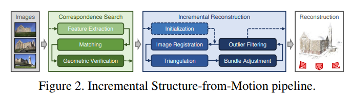
SfM pipeline은 위와 같으며, correspondence search와 incremental reconstruction을 거쳐 최종 reconstruction 결과를 생성한다.

Correspondence Search

SfM의 첫번째 stage로써 correspondence search process는 input image들 $\mathcal I = \{I_i|i=1...N_I\}$에서 scene overlap을 찾아내고, 이러한 overlapping image들에서 같은 projection point들을 찾아낸다.

최종적으로 이 process의 output은 geometrically verified image pair $\bar{\mathcal C}$와 각 point에 대한 image projection의 graph이다.

이 process는 feature extraction / matching / geometric verification process을 포함한다.

Feature Extraction

먼저 각 image $I_i$의 location $x_j\in\mathbb R^2$에서 appearance descriptor $f_j$로 표현되는 local feature set을 추출한다.

이러한 feature는 여러 이미지에서 쉽게 detect되야하므로, radiometric/geometric 변화에 invariant해야 한다.

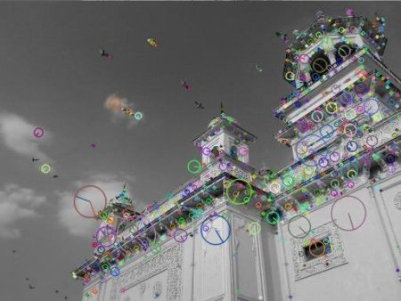
Feature extractor로는 SIFT가 가장 흔히 사용되는 방식이다. SIFT는 간단하게 아래 과정을 통해 feature point를 추출. (Distinctive Image Features from Scale-Invariant Keypoints)

1) Scale-space extrema detection: 다양한 scale에서 극점 찾기
2) Keypoint localization: 극값의 위치 찾기
3) Orientation assignment: keypoint에 방향을 할당
4) Keypoint descriptor: keypoint에 feature 부여

아래 이미지 출처
https://docs.opencv.org/4.x/da/df5/tutorial_py_sift_intro.html

Matching

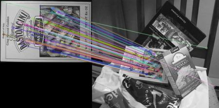
다음으로 SfM은 feature $\mathcal F_i$를 이미지의 appearance description으로 활용해서, 같은 scene part를 보고있는 이미지들을 찾아낸다.

이를 위해 이미지끼리 비슷한 feature들을 searching하여 feature correspondence를 구한다. Feature matching 방법도 다양한게 있다.

Feature matching의 결과로는 overlapping image pair $\mathcal C=\{\{I_a,I_b\} | I_a,I_b \in\mathcal I,a <b\}$와 관련된 feature correspondence $\mathcal M_{ab}\in\mathcal F_a \times\mathcal F_b$를 얻게 된다.

아래 이미지 출처
https://docs.opencv.org/4.x/dc/dc3/tutorial_py_matcher.html

Geometric Verification

세번째로는 위에 Feature matching에서 구한 overlapping image pair $\mathcal C$를 verify한다.

Feature matching stage에서 구한 image pair는 오직 appearance만을 보고 구한 것이기 때문에, matching된 feature들이 실제로 같은 scene point에 mapping된다고 할 수는 없다.

SfM은 projective geometry를 이용해 이미지 사이의 feature point를 mapping하는 transformation을 예측하려고 함으로써 이 match들을 verify한다.

이 작업을 위해 Epipolar geometry의 개념이 필요하다.

Epipolar geometry

참고 자료: https://www.robots.ox.ac.uk/~vgg/hzbook/hzbook2/HZepipolar.pdf

Epipolar geometry는 이미지 pair의 공간적인 configuration에 따라 서로 다른 mapping들 사이의 기하하적 관계를 표현한다.

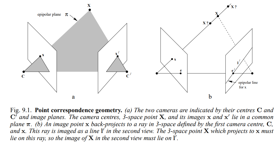
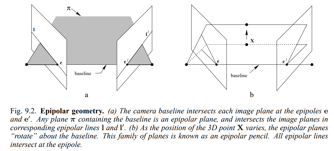
• 두 카메라 $C$ (첫번째 view라고 하자)와 $C'$(두번째 view)와 그의 image plane이 있다고 하자. 3D 공간 상에 점 $X$가 있다면, $X$와 camera center $C$, $C'$, 그리고 image plane 상의 point $x$, $x'$은 하나의 plane $\pi$에 놓이게 되는데, 이를 epipolar plane이라고 한다.

• Image point $x$를 3D space로 back projection하면 $C$와 $x$로 정의된 ray를 생성하는데, 이 ray는 두번째 view에서 $l'$로써 보이게 된다. 즉, 3D space 상의 point $X$는 이 ray위에 위치해야만 하고, 두번째 view에서는 $l'$위에 위치해야한다. 이 $l'$을 x에 대한 epipolar line이라고 한다.

• 각 이미지 image과 camera baseline의 교점을 $e$, $e'$라고 하며, baseline을 포함하는 plane은 모두 epipolar plane이 될 수 있으며, 이는 corresponding epipolar line $l$, $l'$과 만난다.

• 3D point $X$의 위치가 변함에 따라서 epipolar plane은 baseline을 기준으로 rotate하게 된다.

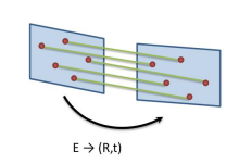
Epipolar geometry에서는 이 두 카메라의 image 내부 대응되는 point끼리의 변환 관계를 essential matrix $E$ (calibrated -> intrinsic matrix를 알때)와 fundamental matrix $F$ (uncalibrated -> intrinsic matrix를 모를 때)로 표현하며, 이러한 변환 행렬은 항상 존재 (Epipolar Constraint)한다.

여러 random matching point를 통해 이러한 matrix를 5-point (essential) / 8-point (fundamental) algorithm를 이용해 estimate하고 이러한 transformation이 두 이미지 사이에 충분히 많은 feature를 matching 시킬 수 있으면, 이를 geometrically verified된 image pair로 생각한다.

이때, least squared method를 이용하면 outlier (실제로 matching되지 않는 point pair)들로 인해 제대로 구해내기가 어려우므로, RANSAC 알고리즘 등을 사용하여 matching point의 feature correspondence에서 outlier를 걸러내는 작업이 동반된다. ->epipolar constraint 값을 계산하고 어떤 threshold를 기준으로 inlier 갯수를 세고 가장 많은 경우를 선택

이 단계에서 output은 아래와 같으며, 이는 image를 node로 하고 verified image pair를 edge로하는 scene graph로도 생각할 수 있다.

• geometrically verified image pairs $\bar \mathcal C$
• associated inlier correspondences $\bar \mathcal M_{ab}$
• (option) description of their geometric relation $G_{ab}$

Incremental Reconstruction

이제 Correspondence search로부터 얻은 scene graph를 이용하여 reconstruction을 수행한다.

• Input: scene graph
• Output
  • Pose estimates $\mathcal P=\{\bold{P}_c\in SE(3) |c=1...N_P\}$ for registered images
  • Reconstructed scene structure as a set of points $\mathcal X=\{\bold{X}_k\in \mathbb R^3|k=1...N_X\}$

이 과정에서는 처음 Initialization 후에, Image Registration / Trigulation / Bundle Adjustment / Outlier Filtering이 계속 반복된다.

Initialization

아주 신중하게 고른 두 개의 image pair를 통해서 reconstruction model을 initialize한다.

Image graph에서 최대한 많은 image와 overlapping되는 위치에서부터 시작하는 것이 제일 좋다고 한다.

Image registration

Incremental reconstruction 과정에서 매번 새로운 image가 현재 model로 register된다. 새로운 이미지를 현재의 3D reconstruction에 추가해주는 것이다.

이는 이미 register된 이미지들에서 triangulated point의 feature correspondence를 이용한 Perspective-n-Point (PnP) problem을 풂으로써 수행하게 된다.

PnP problem은 n개의 2D-3D correspondence (pair)가 주어졌을 때, camera pose를 예측하는 것으로 생각하면 되고, RANSAC 등의 방법을 사용한다.

구해진 pose는 $\mathcal P$에 추가 된다.

---

잠깐만..

나는 여기서의 pose estimation과 geometric verification에서 pose estimation의 역할이 조금 헷갈렸다. 그래서 조금 정리해보자면,

• Epipolar Geometry in the "Verification" Stage
  • Purpose: Epipolar geometry는 초기 단계에서 이미지들 사이의 relative pose를 establish하기 위해 사용된다.
  • Process: Fundamental/Essential matrix를 estimate하고 decompose해서 possible relative pose를 구하고, 추가적인 constraint로 determine
  • Output: 두 이미지 사이의 relative camera pose set -> triangulation process에서 initial image pair에 대한 pose로 활용 된다.
• Perspective-n-Point in the "Image Registration" Stage
  • Purpose: PnP는 실제 우리가 reconstruction하는 3D space에서 camera의 absolute pose를 구하기 위해 사용된다. (예를 들어 첫번째 선택된 카메라의 coordinate를 origin으로 정했다면 그게 recon space)
  • Process: 새 이미지의 feature를 3D space 상의 point와 match 시키고, 이 correspondence를 이용해 camera pose를 estiamte (= PnP)
  • Output: 새로 register된 camera의 absolute pose. 이 pose는 triangulation process에서 이후에 추가되는 image의 pose로 활용된다.

---

Triangulation

새로 register된 image는 반드시 existing scene point를 observe할 수 있어야 한다. 추가적으로 이는 triangulation을 통해 scene structure points $\mathcal X$를 늘릴 수도 있다.

Triangulation은 두 개의 view image에서 함께 보이는 어떤 3D space의 map point를 구해내는 방법이다. 즉 아래와 같이 camera로부터 image를 지나는 두 ray의 교점을 찾는 것이다.

https://www.cs.cmu.edu/~16385/s17/Slides/11.4_Triangulation.pdf

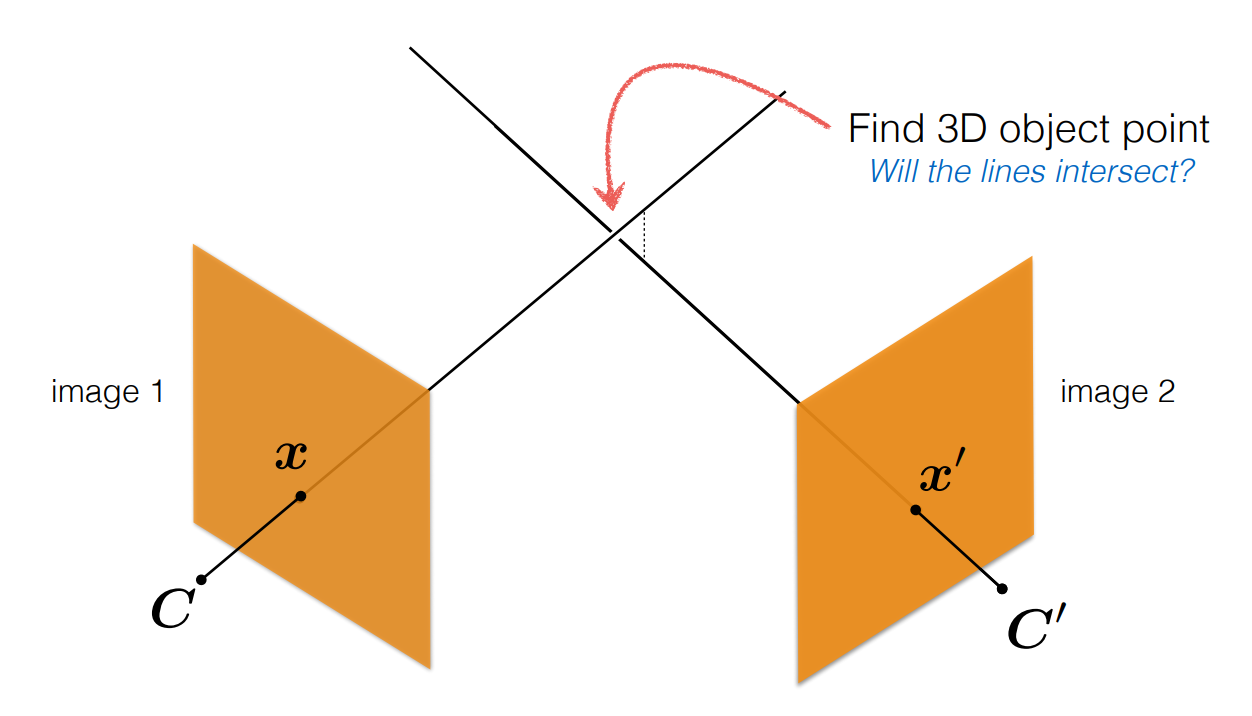
먼저, 우리는 두 이미지 사이의 matching된 point set와 camera pose 정보를 갖고 있다.

이 camera pose는 initial recon step에서는 Epipolar geometry에서 fundamental matrix ($F$)나 essential matrix ($E=K'^TFK$)로부터 얻어낸 pose이고, 이후로는 image registration에서 PnP로 구한 pose이다.

원하는 3D object point를 $X$라고 하자. 각 이미지의 camera projection을 $P_1, P_2$라고 하면

와 같이 표현할 수 있게 되는데, 우리는 $R,t$는 이미 구했고, $K$는 알고 있다고 가정하면,

으로 일단 둘 수 있다. (처음에는 정보가 없으니까, 첫번째 카메라를 그냥 world coordinate system의 origin이라고 가정)

그러면 각 point $x_1, x_2$를 다시 쓸 수 있다.

그런데 여기서 주의할 점이 우리는 projective depth scaling에 대해 고려를 안한 relation matrix만을 알고 있으므로, scale $s_1, s_2$를 고려해서 위 식을 쓰면,

즉, $s_2x_2=s_1Rx_1+t$이 되고, 여기에 $x_2$의 cross product를 사용하여 linear equation을 만들 수 있고, 이를 통해 $s_1, s_2$를 구하면 $X$를 구할 수 있게된다.

실제로는 noise때문에 정확하게 구할 수가 없어서 least-square를 사용한다고 한다.

이렇게 되면 이제 두 이미지에서 하나의 matching point에 대해 3D point를 생성하였다. 이게 모든 matching point에 대해 진행되고, 새로운 이미지가 register될 때마다 또 3D scene point $X_k\in \mathbb R^3$를 계속 생성하게 된다.

** 처음에 첫번째 camera를 world coordinate의 origin으로 가정하고 시작했으므로, 이후에도 모든 3D point는 첫번째 camera coordinate를 기준으로 한다 그게 아니라면 어떤 existing 3D recon space를 가정해도 문제는 없을 것 같다.

Bundle adjustment

출처 https://www.youtube.com/watch?v=EavQ_PodpWQ

---

지금까지의 과정을 정리하면,

우리는 먼저 correspondence searching 과정을 통해 1) 수집된 이미지들의 feature를 추출하고, 2) 그 feature를 matching하여 image pair를 구했다. 3) 다음으론 image pair사이의 relative transformation을 estimation함으로써 geometric verification을 수행하였다.

Incremental reconstruction 과정에서는 처음에 두 장의 이미지에서 시작해서 iteration 마다 새로운 이미지를 추가하면서 계속해서 recon을 이어가는데, 1) 처음에는 두 이미지를 뽑아 첫번째 카메라를 origin으로 가정하고, 두번째 이미지와의 relative transformation를 통해 camera pose를 추출한다. 2) 그리고 이 camera pose와 matching point set을 이용한 triangulation을 통해 주어진 2D coordinate로부터 3D point를 estimation해낸다. 3) 다음으로 추가되는 이미지들은 이전 triangulation에서 얻어진 3D point를 이용한 PnP를 풀어서 camera pose를 구해내며, 4) 다시 이 pose를 활용한 triangulation을 통해 3D point를 계속해서 구해낸다.

---

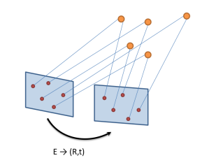
Image registration과 Triangulation은 분리된 process이지만 서로 영향을 크게 주고 받는다. 예를 들어 image registration에서 예측한 pose는 3D point의 triangulation에 직접적으로 영향을 주고 반대로 triangulation에서 예측한 3D point는 image registration에서 pose를 구하는데 영향을 준다.

---

https://www.cs.jhu.edu/~misha/ReadingSeminar/Papers/Triggs00.pdf
에 따르면 bundle adjust의 정의는 다음과 같다.

"Bundle adjustment is the problem of refining a visual reconstruction to produce jointly optimal 3D structure and viewing parameter (camera pose and/or calibration) estimates.

Optimal means that the parameter estimates are found by minimizing some cost function that quantifies the model fitting error, and jointly that the solution is simultaneously optimal with respect to both structure and camera variations.

The name refers to the ‘bundles’ of light rays leaving each 3D feature and converging on each camera centre, which are ‘adjusted’ optimally with respect to both feature and camera positions.

---

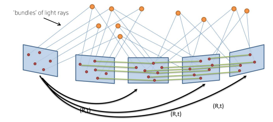
즉, Bundle adjustment는 이전 단계에서 두 장의 image pair에서 pose와 point를 계산한 것과는 다르게, 지금까지 구한 camera pose ($P_c$)와 3D point ($X_k$)를 함께 정제 하고 최적화 (joint non-linear refinement)하는 방법이다.

이는 아래의 reprojection error를 최소화함으로써 수행된다.

Reprojection이라 함은 주어진 3차원 point과 pose를 이용해서 다시 이미지 plane으로 projection 시키는 것이다.

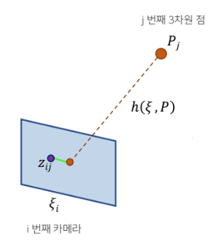
$i$번째 카메라에 대해 $j$번째 3D point를 $i$의 pose를 통해 projection하는 함수를 $h$라고 했을 때, 실제 관측치 $z_{ij}$와의 error를 구하여 이를 최소화 한다.

이 cost function를 최소화하는 방향으로 모든 pose $\xi$와 3D point $p$를 조정해간다.

이를 위해 non-linear optimization을 수행하는데, 초기값을 정하고 위 cost function을 줄이는 방향으로 증가분 ($\Delta \xi, \Delta p$)을 계산하는 방식으로 진행된다.

• 최적화할 변수 : $x=[\xi_1,\xi_2,...,\xi_m, p_1,...,p_m]^T$ <- 모든 pose와 point의 stack

• cost function의 점진적 변화: $e(x+\Delta x)\sim e(x)+J\Delta x$

• Jacobian은 cost function을 pose나 point로 편미분한 것으로 표현

  • $J=[F,E]$ <- $F$는 $e$를 $\xi$로 편미분, $F$는 $e$를 $p$로 편미분
  • $J\Delta x=F_{ij}\Delta\xi_i+E_{ij}\Delta p_j$

• Gauss-Newton이나 Levenberg-Marquardt 등의 방법을 활용하여 계산

이렇게 최종적으로 구한 증가분을 통해서 pose와 3D point를 조정해준다.

Discussion

이번 포스팅을 통해 대략적으로나마 SfM의 흐름에 대해서 이해해보려고 하였다. 이어서 COLMAP이 SfM을 어떻게 더 발전시켰는지에 대해서도 알아볼 것이다.

요즘에는 3D reconstruction을 deep learning을 통해 수행하는 연구가 아주 많고 실제로 성능도 너무 좋다. 필자같은 경우에도 deep learning 기반 방법론들을 먼저 접하고 나서 이 근간이 되는 많은 연구를 조금 더 알아두려고 노력하고 있다.

사실 오히려 deep learning 기반 방법론들이 훨씬 쉽고 간단하게 느껴졌다. 하지만 그런 모델들의 설계에 대해서 더 잘 이해하고, 잘 활용하기 위해서는 기본을 더 이해하는 것이 중요하다고 생각했다.

여전히 SfM에서 사용되는 다양한 계산 도구나 방법론에 대해서는 자세히 다루지 않았다. 물론 그런 것들도 중요하지만, 일단은 흐름과 시스템을 좀 이해하려고 노력했다.

앞으로 3D reconstruction에 대해서 자주 다뤄볼 예정인데, 기회가 될 때마다 차근차근 개념을 쌓아가보자.