import numpy as np
import matplotlib.pyplot as plt
다항함수
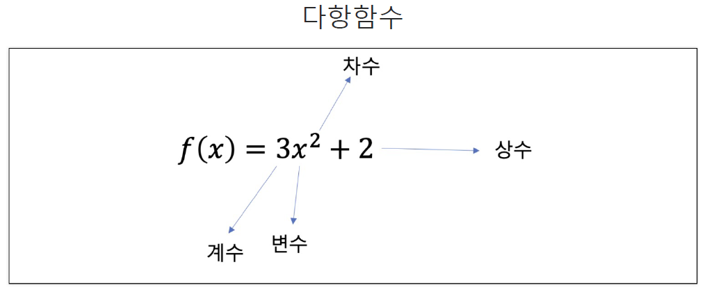
x = np.linspace(-3,2,100)
y = 3 * x**2 + 2
import matplotlib as mpl
mpl.style.use('seaborn-whitegrid')
plt.figure(figsize=(12,8))
plt.plot(x, y)
plt.xlabel('$x$', fontsize=25)
plt.ylabel('$3x^2 +2$', fontsize=25)
plt.show()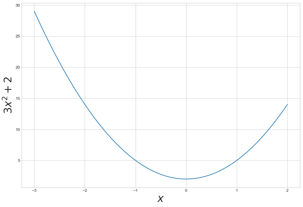
# 다항함수의 x축 방향이동
x = np.linspace(-5,5,100)
y1 = 3*x**2 +2
y2 = 3*(x+1)**2 + 2 #y1의x가 1만큼 이동plt.figure(figsize=(12,8))
plt.plot(x, y1, lw=2, ls='dashed', label='$y=3x^2 +2$') #lw 라벨넓이 ls 라벨스타일
plt.plot(x, y2, label='$y=3(x+1)^2 +2$')
plt.legend(fontsize=15)
plt.xlabel('$x$', fontsize=20)
plt.ylabel('$y$', fontsize=20)
plt.show()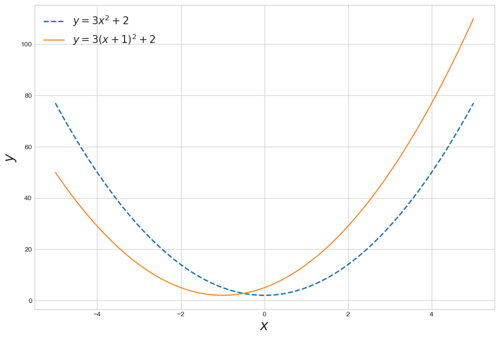
지수함수
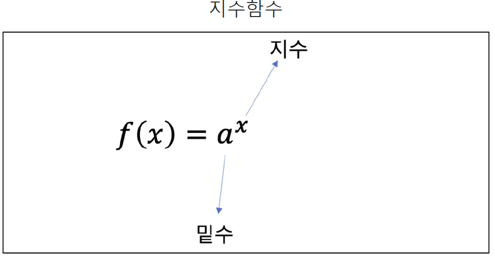
x = np.linspace(-2,2,100)
a11, a12, a13 = 2,3,4
y11, y12, y13 = a11**x, a12**x, a13**x

a21, a22, a23 = 1/2, 1/3, 1/4
y21, y22, y23 = a21**x, a22**x, a23**xfig, ax = plt.subplots(1, 2, figsize=(12,6))
ax[0].plot(x, y11, color='k', label=r"$2^x$") # (1/2)^x = 2^-x
ax[0].plot(x, y12, '--', color='k', label=r"$3^x$")
ax[0].plot(x, y13, ':', color='k', label=r"$4^x$")
ax[0].legend(fontsize=20)
ax[1].plot(x, y21, color='k', label=r"$(1/2)^x$")
ax[1].plot(x, y22, '--', color='k', label=r"$(1/3)^x$")
ax[1].plot(x, y23, ':', color='k', label=r"$(1/4)^x$")
ax[1].legend(fontsize=20)
plt.show()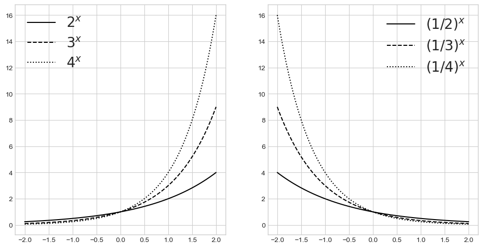
지수증가
plt.figure(figsize=(6,6))
x =np.linspace(0,10)

plt.plot(x, x**2, '--', color='k', label=r'$x^2$')
plt.plot(x, 2**x, color='k', label=r'$2^x$')

plt.legend(loc='center left', fontsize=25)
plt.xlabel('$x$', fontsize=20)
plt.ylabel('$y$', fontsize=20)
plt.show()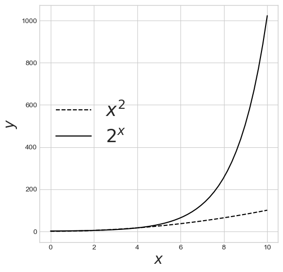
# 2.718..특정 값으로 점점 수렴하는 특징
x = np.array([10, 100, 1000, 10000, 100000, 1000000])

(1+ 1/x)**x
array([2.59374246, 2.70481383, 2.71692393, 2.71814593, 2.71826824,
2.71828047])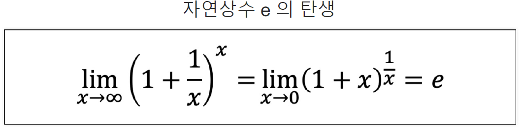
# 자연상수 e
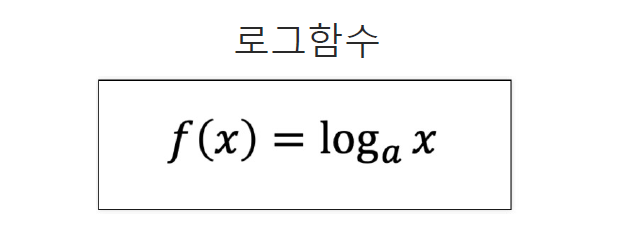
np.exp(1)2.718281828459045로그함수
#로그함수 그리는 데이터
def log(x, base):
    return np.log(x)/np.log(base)

x1 = np.linspace(0.0001, 5, 1000)
x2 = np.linspace(0.01, 5, 100)

y11, y12 = log(x1, 10), log(x2, np.e)
y21, y22 = log(x1, 1/10), log(x2, 1/np.e)fig, ax = plt.subplots(1, 2, figsize=(12,6))
ax[0].plot(x1, y11, color='k', label='$\log_{10} x$')
ax[0].plot(x2, y12, '--',color='k', label='$\log_{e} x$')
ax[0].set_xlabel('$x$', fontsize=25)
ax[0].set_ylabel('$y$', fontsize=25)
ax[0].legend(fontsize=20, loc='lower right')
ax[1].plot(x1, y21, color='k', label='$\log_{1/10} x$')
ax[1].plot(x2, y22, '--',color='k', label='$\log_{1/e} x$')
ax[1].set_xlabel('$x$', fontsize=25)
ax[1].set_ylabel('$y$', fontsize=25)
ax[1].legend(fontsize=20, loc='upper right')
plt.show()
#로그함수의 특성 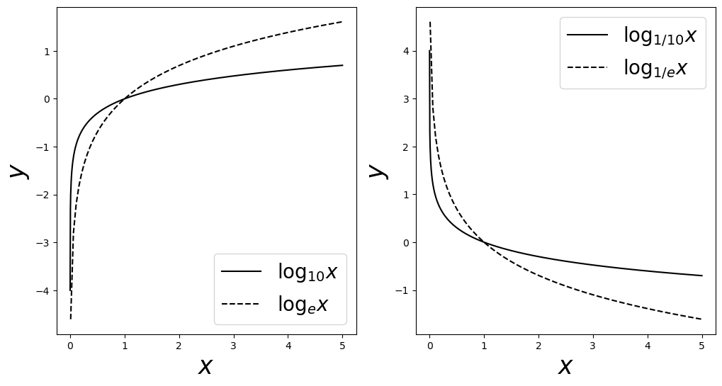
시그모이드 함수
# 시그모이드는 0과 1 사이의 값을 가짐.

z = np.linspace(-10, 10, 100)
sigma = 1/(1+np.exp(-z))

plt.figure(figsize=(12,8))
plt.plot(z, sigma)
plt.xlabel('$z$', fontsize=25)
plt.ylabel('$\sigma(z)$', fontsize=25)

plt.show()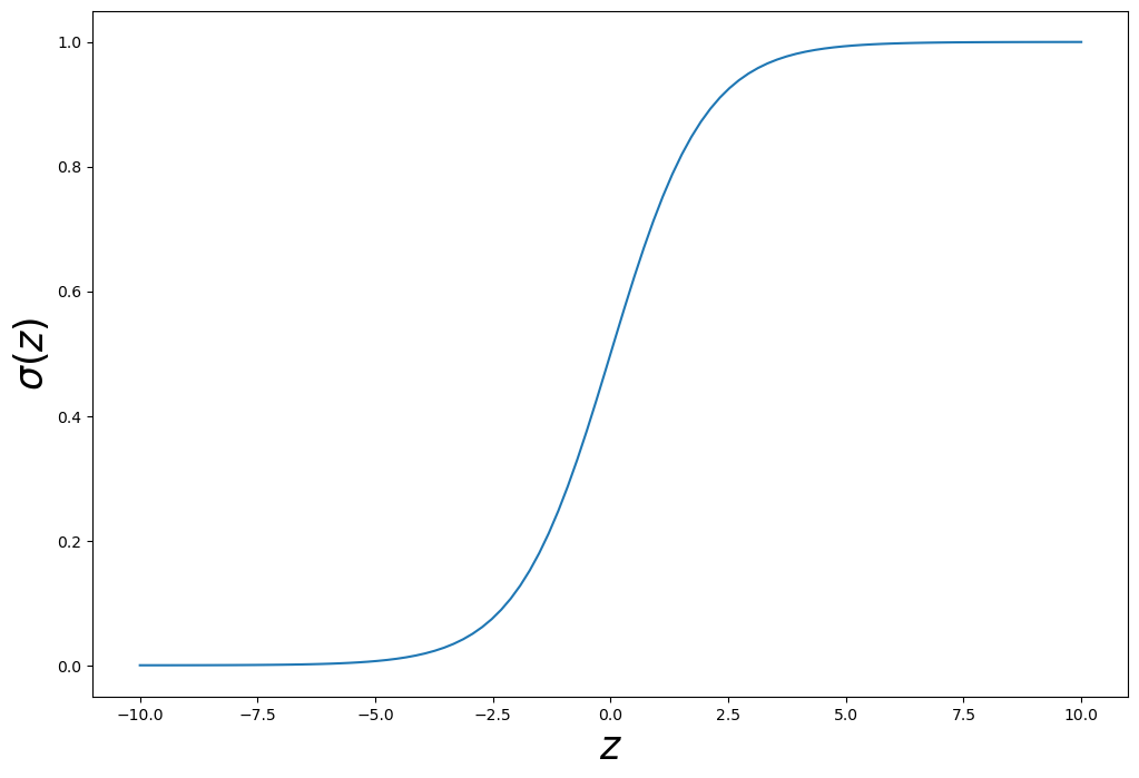

데이터분석 스터디노트🧐✍️