◾PYTORCH 기초
PyTorch: Python을 위한 오픈소스 머신 러닝 라이브러리
import torch- 일반적인 python 코드
x = 3.5
y = (x-1) * (x-2) * (x-3)
print(x, y)
- torch 코드
- 계산을 위한 값을
torch.tensor로 선언한다. requires_grad = True옵션으로 기울기를 찾을 수 있다.
- 계산을 위한 값을
x = torch.tensor(3.5, requires_grad=True)   # 숫자 배치
y = (x-1) * (x-2) * (x-3)
print(x, y)
기울기 찾기
y.backward()
x.grad
- torch로 미분 계산하기
a = torch.tensor(2.0, requires_grad=True)
b = torch.tensor(1.0, requires_grad=True)

x = 2*a + 3*b
y = 5*a*a + 3*b*b*b
z = 2*x + 3*y
z.backward()
a.grad
◾보스톤 집값 예측
- 데이터 준비
- 보스톤 집값 데이터
import pandas as pd
import seaborn as sns
import matplotlib.pyplot as plt
from sklearn.datasets import load_boston

boston = load_boston()
print(boston.DESCR)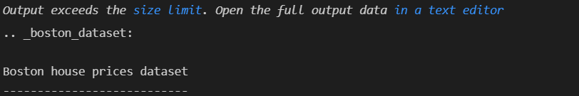
# 데이터 준비
df = pd.DataFrame(boston.data, columns = boston.feature_names)
df['TARGET'] = boston.target
df.tail()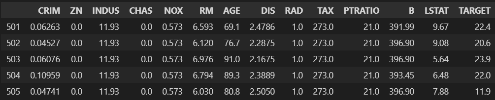
- torch 모듈
import torch
import torch.nn as nn
import torch.nn.functional as F
import torch.optim as optim
- 데이터 분리
- torch는 numpy를 주로 사용한다.
cols = ["TARGET", "INDUS", "RM", "LSTAT", "NOX", "DIS"]
data = torch.from_numpy(df[cols].values).float()
data.shape
data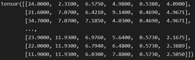
- 특성과 라벨 분리
y = data[:, :1]
x = data[:, 1:]

print(x.shape, y.shape)
- 하이퍼파라미터 설정
n_epochs = 2000
learning_rate = 1e-3
print_interval = 100
- 모델 수립
model = nn.Linear(x.size(-1), y.size(-1))
model
optimizer = optim.SGD(model.parameters(), lr=learning_rate)- 학습 시작
- tensorflow와 달리 for문을 통해 직접 진행한다.
for i in range(n_epochs):
    y_hat = model(x)
    loss = F.mse_loss(y_hat, y)

    optimizer.zero_grad()
    loss.backward()

    optimizer.step()

    if (i + 1) % print_interval == 0:
        print('Epoch %d: loss = %.4e' % (i+1, loss))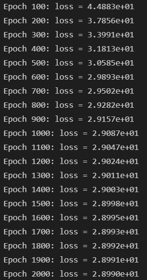
- 학습 결과 정리
df = pd.DataFrame(torch.cat([y, y_hat], dim=1).detach_().numpy(),
                  columns=["y", "y_hat"])
sns.pairplot(df, height=5)
plt.show()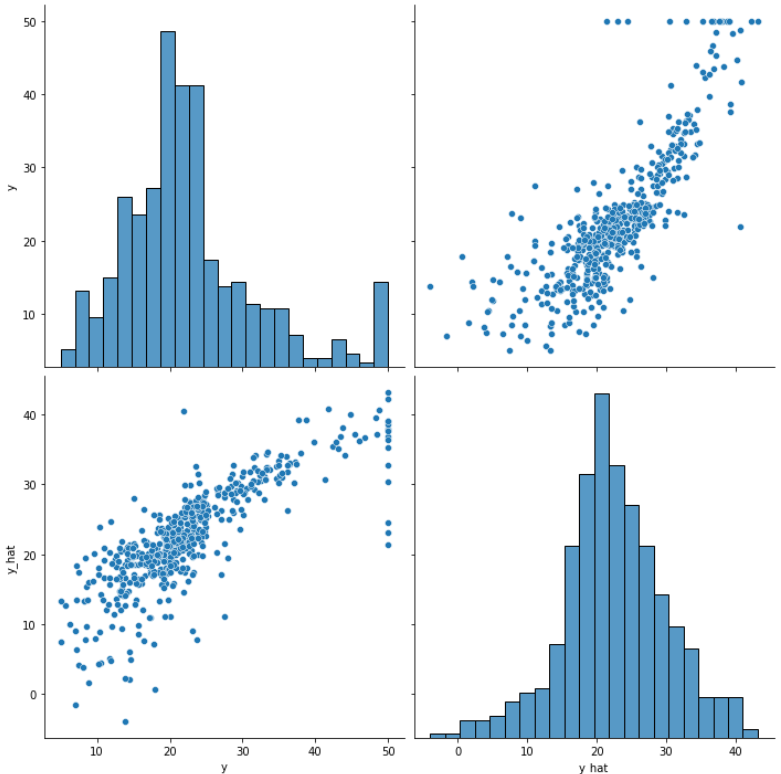
◾유방암 예측
- 데이터 준비
- 유방암 데이터
import pandas as pd
import seaborn as sns
import matplotlib.pyplot as plt
from sklearn.datasets import load_breast_cancer

cancer = load_breast_cancer()
print(cancer.DESCR)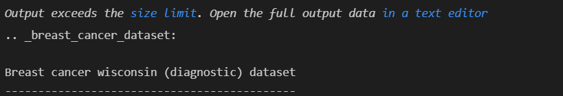
# 데이터 준비
df = pd.DataFrame(cancer.data, columns = cancer.feature_names)
df['class'] = cancer.target
df.tail()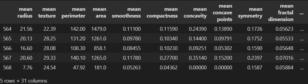
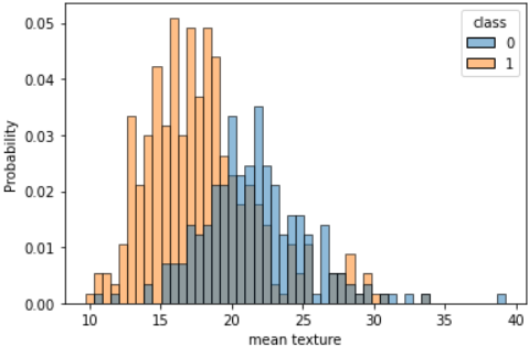
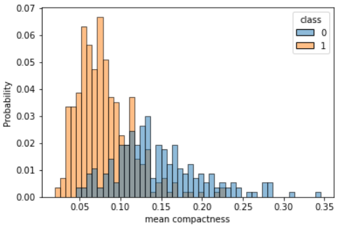
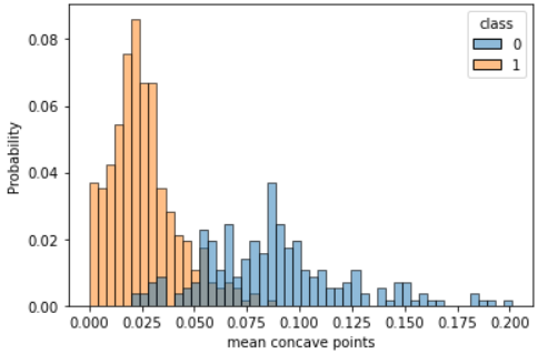
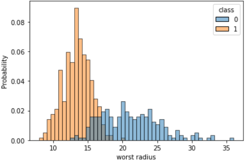
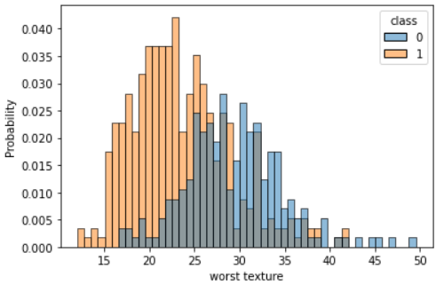
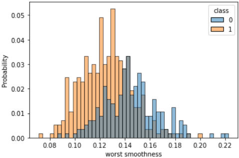
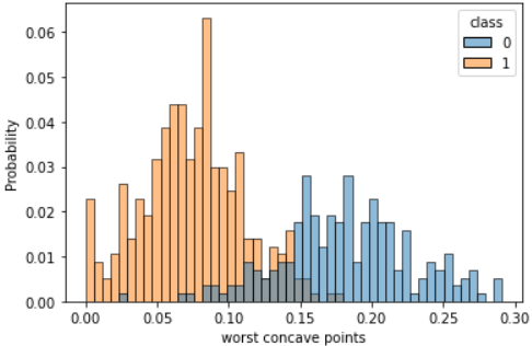
- 관심 컬럼 선정
cols = ["mean radius", "mean texture", "mean smoothness", 'mean compactness',
        'mean concave points', 'worst radius', 'worst texture', 'worst smoothness',
'worst compactness', 'worst concave points', 'class']- 각 컬럼의 histogram 확인
for c in cols[:-1]:
    sns.histplot(df, x=c, hue=cols[-1], bins=50, stat='probability')
    plt.show()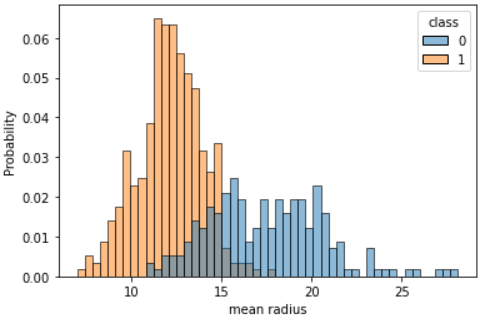


- torch 모듈
import torch
import torch.nn as nn
import torch.nn.functional as F
import torch.optim as optim
- 데이터 분리
- torch는 numpy를 주로 사용한다.
data = torch.from_numpy(df[cols].values).float()
data.shape
data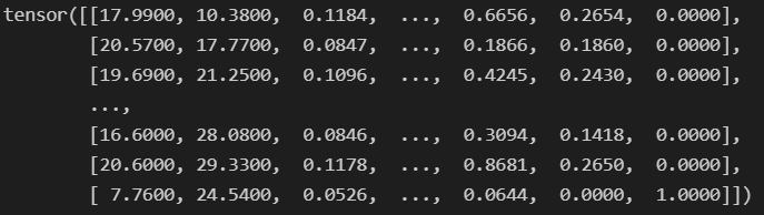
- 특성과 라벨 분리
x = data[:, :-1]
y = data[:, -1:]

print(x.shape, y.shape)
- 하이퍼파라미터 설정
n_epochs = 200000
learning_rate = 1e-2
print_interval = 10000
- 모델 수립
# class로 구성
class MyModel(nn.Module):
    def __init__(self, input_dim, output_dim):
        # input, output 초기화
        self.input_dim = input_dim
        self.output_dim = output_dim

        # 모델 초기화
        super().__init__()

        # Linear 구성
        self.linear = nn.Linear(input_dim, output_dim)

        # activation Func : Sigmoid
        self.act = nn.Sigmoid()

    def forward(self, x):
        # |x| = (batch_size, input_dim)
        y = self.act(self.linear(x))
        # |y| = (batch_size, output_dim)
        return y

model = MyModel(input_dim=x.size(-1), output_dim=y.size(-1))
crit = nn.BCELoss() # Define BCELoss instead of MSELoss
optimizer = optim.SGD(model.parameters(), lr=learning_rate)
- 학습 시작
for i in range(n_epochs):
    y_hat = model(x)
    loss = crit(y_hat, y)

    optimizer.zero_grad()
    loss.backward()

    optimizer.step()

    if (i + 1) % print_interval == 0:
        print('Epoch %d: loss = %.4e' % (i+1, loss))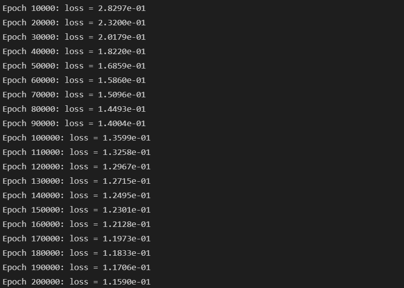
- acc 계산
- 출력으로 sigmoid를 사용했으므로 값으 0 ~ 1 사이를 지닌다.
- 0.5보다 클 경우를 1, 작을 경우를 0으로 바꾸어 실제 값과 비교한다.
- 맞춘 결과과 실제 크기로 Acc를 구한다.
correct_cnt = (y == (y_hat > .5)).sum()
total_cnt = float(y.size(0))

print('Accuracy : %.4f' % (correct_cnt / total_cnt))
- 학습 결과 정리
df = pd.DataFrame(torch.cat([y, y_hat], dim=1).detach().numpy(),
                  columns=["y", "y_hat"])
sns.histplot(df, x='y_hat', hue='y', bins=50, stat='probability')
plt.show()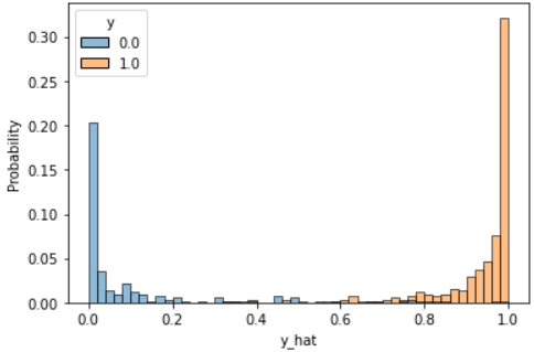

후라이드 치킨