◾Cost Function
1. Cost Function 개념
Cost Function: 원래의 값과 가장 오차가 작은 가설함수 를 도출하기 위해 사용되는 함수- 가설 함수의 형태를 결정짓는 것은
매개변수 - 선형 회귀의 경우 :
- 최소값을 가지는 을 찾는 것이 목표
- 가설 함수의 형태를 결정짓는 것은
- 회귀 +
Cost Function지도학습을 통해 연속된 값을 예측하는회귀- 데이터 -> (학습 데이터셋 + 학습 알고리즘 : 모델 학습) : 가설 -> 예측(결과)
- Hypothesis(가설 = 모델) : h
- 선형 회귀일 경우 :
- 직선으로만 표현한다면 각 점(데이터)과 직선 사이의 에러가 작아지도록 구성할 것이다.
MSE(Min Squared Error): 각 에러의 제곱의 평균을 구한다(부호를 없애기 위해 제곱 사용, 절대값으로 하는 경우도 있다.)- MSE를 구하는 것이
Cost Function: 에러를 표현하는 도구, 값이 작을 수록 좋은 것 - Cost Function의 최소화할 수 있따면 최적의 직선을 찾을 수 있다.
# Cost Function
import numpy as np

# 값의 간결함을 위해 평균대신 합으로 표현
# 실제라면 평균으로 한다는 것 주의!
np.poly1d([2, -1]) ** 2 + np.poly1d([3, -5]) ** 2 + np.poly1d([5, -6]) ** 2
- Cost Funtion :
# 그래프 그리기
import matplotlib.pyplot as plt
import set_matplotlib_korean

x = np.arange(-3, 6, 0.1)
y = 38*(x**2) - 94*x + 62

plt.figure(figsize=(7, 5))
plt.plot(x, y)
plt.grid()
plt.xlim([-3, 6])
plt.show()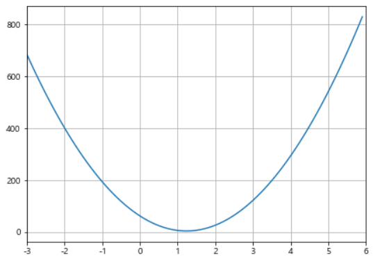
- Cost Function 최소값 찾기 : 미분 사용
# Cost Function 최소값 구하기
# Symbolic 연산 사용
import sympy as sym
theta = sym.Symbol('theta')
# diff(식, 미분할 변수) : 미분 함수
diff_th = sym.diff(38*(theta**2) - 94*theta + 62, theta)
print(94 / 76)
diff_th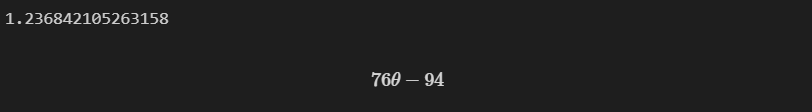
2. Cost Function과 Gradient descent
- 실제 데이터는 복잡하여 손으로 풀기 어렵다
- 데이터의 특징(feature)이 여러개가 존재하여 평면상의 방정식이 아니라
다차원에서 고민해야할 때가 많다. - Cost Function이 최소값을 가지는 지점을 어떻게 찾아야할까
Gradient Descent:- 임의의 점 선택
- 임의의 점에서 미분(or 편미분)값을 계산해 업데이트 : (단, )
- 최소값 기준 왼쪽이든, 오른쪽이든 점점 최소값에 가까워진다.
- 학습률(Learning Rate) : - 얼마만큼 theta를 갱신할 것인지를 설정하는 값
- 적당한 값을 찾아야하는
하이퍼 파라미터중 하나
- 적당한 값을 찾아야하는
- 다변수 데이터에 대한 회귀
- 여러개의 특성(feature)을 가진 경우
Multivariate Linear Regression문제로 일반화할 수 있다.
- 여러개의 특성(feature)을 가진 경우
◾ Bostone 집값 예측
개요
- 보스톤 집 가격 데이터 : Carnegie Mellon University에서 유지 관리
- 회귀 문제를 다루는 많은 머신 러닝 논문에서 사용
데이터 정리
# 데이터 읽기
from sklearn.datasets import load_boston

boston = load_boston()
print(boston.DESCR)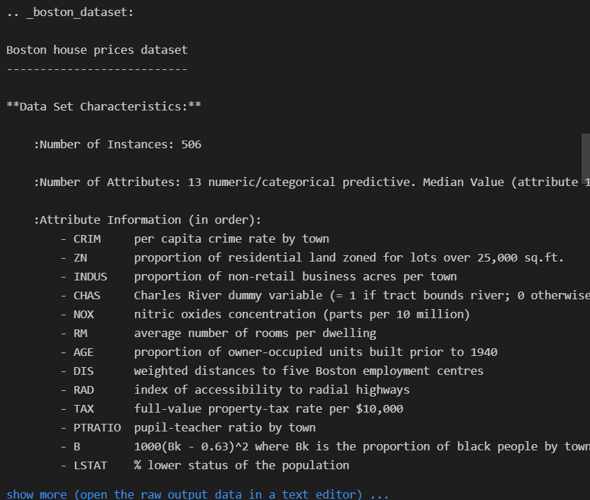
- boston 특성(컬럼) 확인
- CRIM 범죄율
- ZN 25,000 평방 피트 초과 거주지역 비율
- INDUS 비소매상업지역 면적 비율
- CHAS 찰스강의 경계에 위치한 경우는 1, 아니면 0
- NOX 일산화질소 농도
- RM 주택당 방 수
- AGE 1940년 이전에 건축된 주택의 비율
- DIS 직업 센터의 거리
- RAD 방사형 고속도로까지의 거리
- TAX 재산세율
- PTRATIO 학생/교사 비율
- B 인구 중 흑인 비율
- LSTAT 인구 중 하위 계층 비율
# DataFrame 형식으로 변경
import pandas as pd
boston_df = pd.DataFrame(boston.data, columns=boston.feature_names)
# PRICE 컬럼은 Label이므로 주의해서 다루어야한다.
boston_df['PRICE'] = boston.target

boston_df.head()
# Price에 대한 histogram
import plotly.express as px

fig = px.histogram(boston_df, x='PRICE')
fig.show()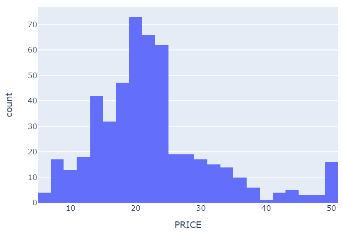
PRICE에 대한 결과를 보면RM(방의 수),LSTAT(저소득층 인구)와 높은 상관관계를 확인할 수 있다.
# 상관계수 조사
import matplotlib.pyplot as plt
import seaborn as sns

corr_mat = boston_df.corr().round(1)
plt.figure(figsize=(12, 7))
sns.heatmap(data=corr_mat, annot=True, cmap='bwr')
plt.show()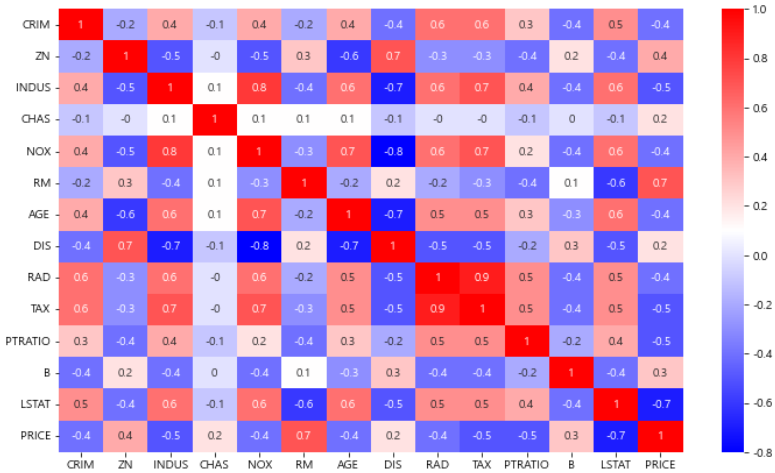
- 일반적으로 방이 많을 수록 집 값이 높아진다.
- 일반적으로 저소득층 인구가 적을 수록 집 값이 높아진다.
- 저소득층이 집값이 낮은 곳을 찾는 것인지
- 저소득층이 살아서 집값이 낮아지게 된 것인지
- 어떤 의미를 지는지 정확히 파악할 수 없다.. 이런 부분은 본인의 고민이 필요한 부분이다
# RM과 LSTAT와 PRICE의 관계 조금 더 관찰
sns.set_style('darkgrid')
sns.set(rc={'figure.figsize' : (12, 6)})
fig, ax = plt.subplots(ncols=2)
sns.regplot(x='RM', y='PRICE', data=boston_df, ax=ax[0])
sns.regplot(x='LSTAT', y='PRICE', data=boston_df, ax=ax[1])
plt.show()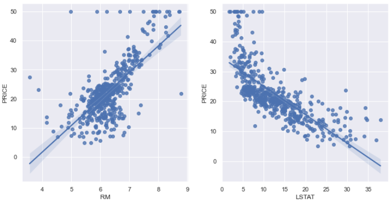
예측 모델
모든 특성 사용
# 데이터 나누기
from sklearn.model_selection import train_test_split

X = boston_df.drop('PRICE', axis=1)
y = boston_df['PRICE']

X_train, X_test, y_train, y_test = train_test_split(X, y, test_size=0.2, random_state=13)
# 선형 회귀 학습
from sklearn.linear_model import LinearRegression
reg = LinearRegression()
reg.fit(X_train, y_train)# 모델 평가 : RMS(Root Mean Square) 사용
import numpy as np
from sklearn.metrics import mean_squared_error
pred_tr = reg.predict(X_train)
pred_test = reg.predict(X_test)
rmse_tr = (np.sqrt(mean_squared_error(y_train, pred_tr)))
rmse_test = (np.sqrt(mean_squared_error(y_test, pred_test)))
print('RMSE of Train Data : {}'.format(rmse_tr))
print('RMSE of Test Data : {}'.format(rmse_test))
# 성능 확인 : 직선에 모일 수록 좋은 성능을 가진 것이다.
plt.figure(figsize=(10, 6))
plt.scatter(y_test, pred_test)
plt.xlabel('Actual House Prices ($1000)')
plt.ylabel('Predicted Prices')
plt.title('Real vs Predicted')
plt.plot([0, 48], [0, 48], 'r')
plt.show()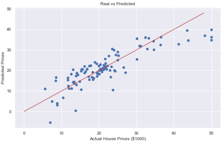
LSTAT 제외
# 데이터 나누기
from sklearn.model_selection import train_test_split

X = boston_df.drop(['PRICE', 'LSTAT'], axis=1)
y = boston_df['PRICE']

X_train, X_test, y_train, y_test = train_test_split(X, y, test_size=0.2, random_state=13)
# 선형 회귀 학습
from sklearn.linear_model import LinearRegression
reg = LinearRegression()
reg.fit(X_train, y_train)# 모델 평가 : RMS(Root Mean Square) 사용
import numpy as np
from sklearn.metrics import mean_squared_error
pred_tr = reg.predict(X_train)
pred_test = reg.predict(X_test)
rmse_tr = (np.sqrt(mean_squared_error(y_train, pred_tr)))
rmse_test = (np.sqrt(mean_squared_error(y_test, pred_test)))
print('RMSE of Train Data : {}'.format(rmse_tr))
print('RMSE of Test Data : {}'.format(rmse_test))
# 성능 확인 : 직선에 모일 수록 좋은 성능을 가진 것이다.
plt.figure(figsize=(10, 6))
plt.scatter(y_test, pred_test)
plt.xlabel('Actual House Prices ($1000)')
plt.ylabel('Predicted Prices')
plt.title('Real vs Predicted')
plt.plot([0, 48], [0, 48], 'r')
plt.show()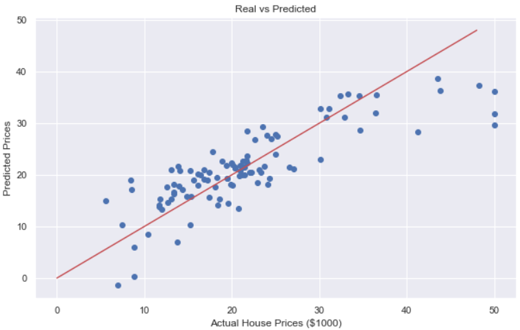

후라이드 치킨