머신 러닝 - Iris Classification(3)

◾데이터 나누기(Decision Tree)

1. 과적합

• 과적합(Overfitting) : 기계 학습(machine learning)에서 학습 데이터를 과하게 학습(overfitting)하는 것을 뜻한다. 일반적으로 학습 데이타는 실제 데이타의 부분 집합이므로 학습데이타에 대해서는 오차가 감소하지만 실제 데이터에 대해서는 오차가 증가하게 된다.
• 지도 학습 : 학습 대상이 되는 데이터에 정답을 붙여서 학습시키고 모델을 얻어 완전히 새로운 데이터에 대한 '답'을 얻고자 하는 것
  • 학습, 추론(학습된 모델을 사용하는 것)
• 이전 포스트에서 만든 Decision Tree를 확인하면 복잡한 규칙으로 이루어진 것을 볼 수 있다.

# decision tree 그래프
from sklearn.tree import plot_tree

plt.figure(figsize=(12, 8))
plot_tree(iris_tree)
plt.show()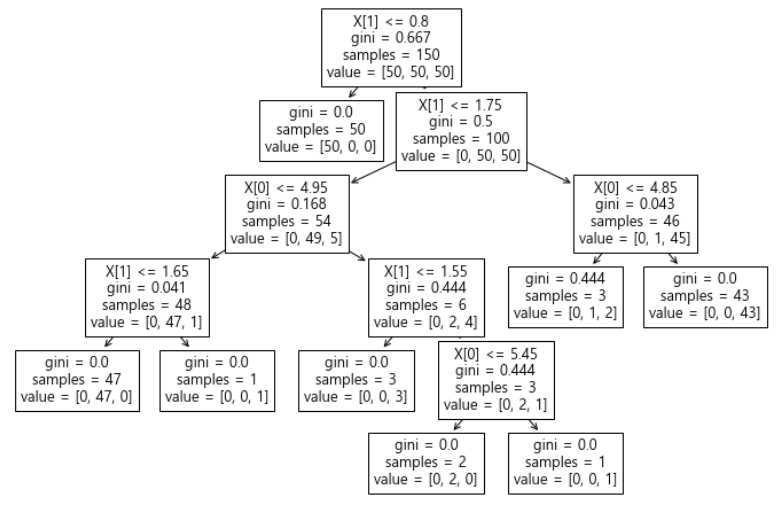

• mlxtend : sklearn에 없는 몇몇 기능을 가지고 있다.

# 결정나무 모델이 어떻게 데이터를 분류했는지 확인할 수 있다.
from mlxtend.plotting import plot_decision_regions

plt.figure(figsize=(14, 8))
plot_decision_regions(X=iris.data[:, 2:], y=iris.target, clf=iris_tree, legend=2)
plt.show()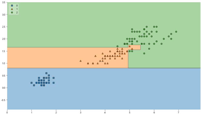

• 조건이 복잡하게 결정된 것을 알 수 있다.
• 모든 IRIS에 대해 맞는 경계선을 가질 수 있는가?
• 이 결과를 내가 가진 데이터를 벗어나서 일반화할 수 있는가
• 얻은 데이터는 유한하고 얻은 데이터를 이용해 일반화를 추구하게 된다.
• 복잡한 경계면은 모델의 성능을 결국 나쁘게 만든다.

2. 데이터 분리(나누기)

• 데이터의 분리 : 훈련(Training), 검증(Validation), 평가(Testing)
  • 확보한 데이터 중에서 모델 학습에 사용하지않고 빼둔 데이터를 이용해 모델 테스트

import pandas as pd
import numpy as np
from sklearn.datasets import load_iris
from sklearn.model_selection import train_test_split
from sklearn.tree import DecisionTreeClassifier

iris = load_iris()

features = iris.data[:, 2:]
labels = iris.target

# 랜덤으로 데이터를 선택하기 때문에 라벨간 비율이 맞지않을 수 있다.
# X_train, X_test, Y_train, Y_test = train_test_split(features, labels, test_size=0.2, random_state=318)
# 라벨간 비율을 맞추기 위해 stratify 옵션 사용
X_train, X_test, Y_train, Y_test = train_test_split(features, labels, 
                                                    test_size=0.2, 
                                                    stratify=labels,
                                                    random_state=13)

# train 데이터를 대상으로 결정 나무 모델 생성
# 학습의 일관성을 위해 random_state 고정
# 모델의 단순화를 위해 max_depth 조정 => 규제
iris_tree = DecisionTreeClassifier(max_depth=2, random_state=13)
iris_tree.fit(X_train, Y_train)

# 트리(모델) 확인
import matplotlib.pyplot as plt
from sklearn.tree import plot_tree

plt.figure(figsize=(12, 10))
plot_tree(iris_tree)
plt.show()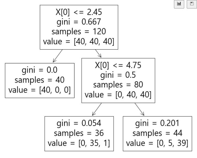

# 정확성 계산
# iris 데이터가 단순해서 높은 정확성을 보인다.
from sklearn.metrics import accuracy_score

y_pred_tr = iris_tree.predict(X_train)
accuracy_score(Y_train, y_pred_tr)

# 결정 경계 확인
import matplotlib.pyplot as plt
from mlxtend.plotting import plot_decision_regions

plt.figure(figsize=(12, 8))
plot_decision_regions(X=X_train, y=Y_train, clf=iris_tree, legend=2)
plt.show()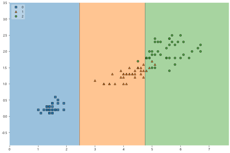

# 테스트 데이터에 대한 accuracy
y_pred_test = iris_tree.predict(X_test)
accuracy_score(Y_test, y_pred_test)

# 테스트 데이터 결정 경계 확인
import matplotlib.pyplot as plt
from mlxtend.plotting import plot_decision_regions

scatter_highlight_kwargs = {'s' : 150, 'label' : 'Test data', 'alpha' : 0.9}
scatter_kwargs = {'s' : 120, 'edgecolor' : None, 'alpha' : 0.9}

plt.figure(figsize=(12, 8))
plot_decision_regions(X=features, y=labels,
                      X_highlight=X_test, clf=iris_tree, legend=2,
                      scatter_highlight_kwargs = scatter_highlight_kwargs,
                      scatter_kwargs = scatter_kwargs,
                      contourf_kwargs={'alpha' : 0.2}
                      )
plt.show()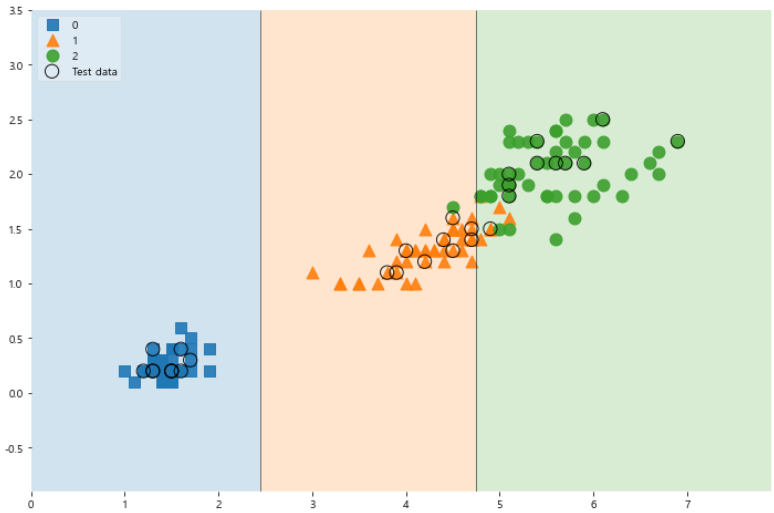

# feature 4개 사용
features = iris.data
labels = iris.target

x_train, x_test, y_train, y_test = train_test_split(features, labels,
                                                    test_size = 0.2,
                                                    stratify = labels,
                                                    random_state=13)

iris_tree = DecisionTreeClassifier(max_depth = 2, random_state = 13)
iris_tree.fit(x_train, y_train)

# 결정 트리 확인
plt.figure(figsize=(12, 10))
plot_tree(iris_tree)
plt.show()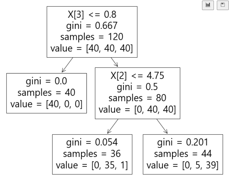

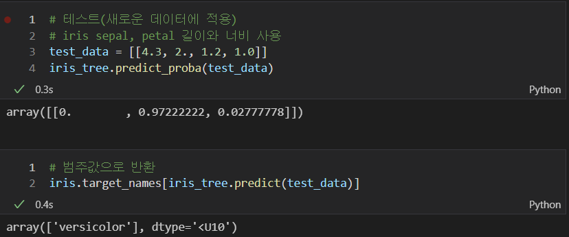
• 구현한 모델 테스트
  
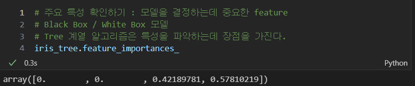
• 구현 모델의 특성