GeNeVA-GAN

김상현·2020년 12월 22일

해당 글은 GeNeVA-GAN 논문 리뷰로 빅데이터 연합동아리 tobigs 생성모델 세미나 자료로 사용되었습니다.

Tell,Draw,and Repeat: Generating and Modifying Images Based on Continual Linguistic Instruction

Introduction

GeNeVA는 Generative Neural Visual Artist로 빈 캔버스에 점진적으로 그림을 그리는 과정에 영감을 받았다. 주어진 caption(사진 삽화에 붙은 설명)에 따라 이미지를 만드는 것이 아닌 continual linguistic 입력을 기반으로 반복적으로 이미지를 생성한다.

Task and Datasets

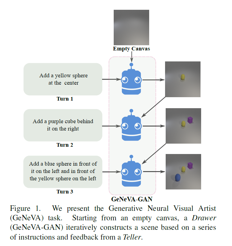
GeNeVA는 Teller와 Drawer가 존재한다. Teller는 지시를 하고, Drawer는 지시에 맞게 캔버스에 그림을 반복적으로 그려나간다. Teller는 Drawer가 생성한 이미지를 통해 전체 과정의 진전을 판단하다. Drawer는 지시에 맞는 물체를 물체의 특성을 잘 살리면서 또한 물체들간의 위치를 고려하여 이미지를 생성해야 한다. Drawer는 또한 이전의 이미지와 지시를 유지하는 방식으로 이미지를 수정해 나가야한다. 따라서 이전의 이미지와 지시를 기억하고 있어야 한다.

사용한 데이터셋은 CoDraw dataset과 CLEVR dataset을 iterative하게 변형시킨 i-CLEVR dataset을 이용했다.

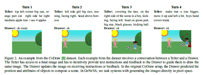
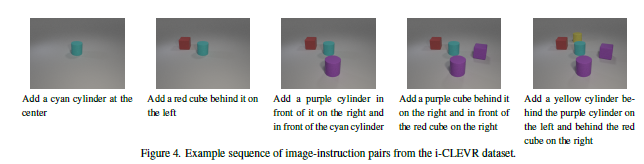
CoDraw dataset과 i-CLEVR dataset 예시

두 dataset 모두 합성 이미지(실제 사진과 같은 이미지가 아닌)들로 구성된 dataset이다. 해당 논문의 저자들은 "합성 이미지를 통해 모델의 성능을 향상시킬 수 있었고, 사실적인 이미지(사진)는 더욱 도전적인 작업이지만, 이 모델은 합성 이미지를 생성하는데만 국한되지 않는다"고 밝혔다.

Contributions

Instruction history의 맥락에서 이미지의 그럴듯한 수정에 특화된 새로운 recurrenct GAN을 제안한다.
i-CLEVR dataset을 소개한다.
지시에 합당한 위치에 물체들을 위치시키는 능력을 평가하기 위해 rsim(relationship similarity) metric을 제안한다.
비반복적 생성 모델과 비교하며 반복적 생성 모델의 중요성을 설명한다.

Model

notation
$x_{0}$ : canvas
Q = ( $q_{1}$ ,..., $q_{n}$ ): sequence of instructions
G/D: generator/discriminator
R: second GRU
$E_{G}$ : image encoder(shallow CNN)
$E_{D}$ : image encoder for discriminator
$z_{t}$ : a noise vector sampled from N(0,1)
$h_{t}$ : context-aware condition
$f_{G_{t-1}}$ : context-free condition
$x_{t}$ : ground-truth image
$\tilde{x}_{t}$ : generated image

Generator part

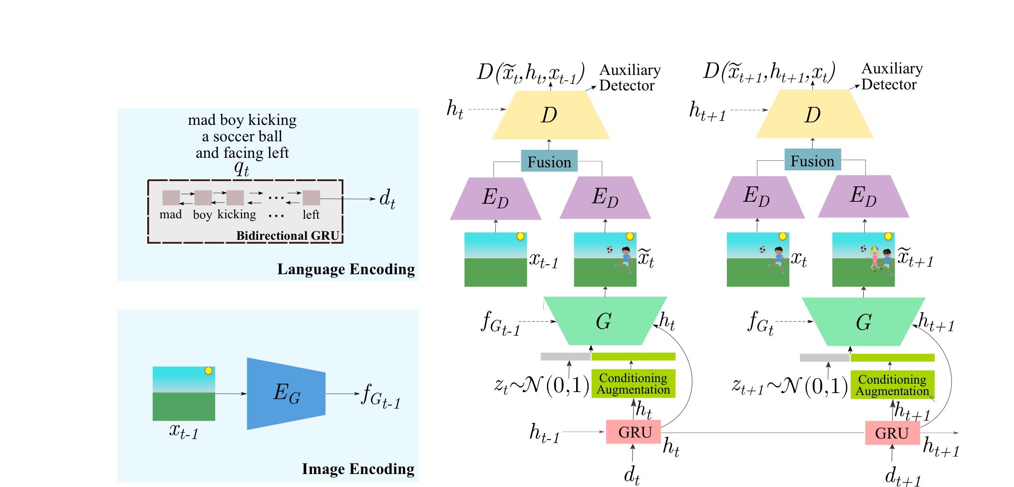
t 시점의 합성된 이미지 $\tilde{x}_{t}$ = G( $z_{t}$ , $h_{t}$ , $f_{G_{t-1}}$ )
먼저 generator의 각 입력들에 대해 알아보자.

$z_{t}$ 는 위의 notation과 마찬가지로 t 시점의 noise vector이다.
$h_{t}$ 는 context-aware condition으로 $h_{t}$ = R( $d_{t}$ , $h_{t-1}$ ) 이다. 먼저 $d_{t}$ 는 t 시점의 instruction $q_{t}$ 를 bi-directional GRU GloVe word embedding을 이용해 인코딩 된 벡터이다. 따라서 $h_{t}$ 는 instruction encoding $d_{t}$ 와 t-1시점의 context-aware condition $h_{t-1}$ 을 입력으로 받아 R(GRU)를 통과하여 현 시점의 정보(insturction)와 이전 시점의 정보(instruction)를 종합하여 새로운 이미지를 그리는데 수정해야할 부분을 나나태는 벡터이다.
$f_{G_{t-1}}$ 은 context-free condition으로 $f_{G_{t-1}}$ = $E_{G}$ ( $\tilde{x}_{t-1}$ )이다. 이전 시점에 생성된 이미지를 인코딩하여 현재 캔버스의 정보를 나타내는 벡터이다.

다음으로 t 시점의 합성된 이미지 $\tilde{x}_{t}$ 가 합성되는 과정을 확인하자.
1. t 시점의 instruction $q_{t}$ 를 language encoder를 통해 $d_{t}$ 를 생성
2. R( $d_{t}$ , $h_{t-1}$ )을 통해 $h_{t}$ 생성
3. $z_{t}$ 와 conditioning augmentation을 통한 $h_{t}$ 를 concat하여 noise vector 생성
4. t-1 시점의 이미지를 image encoder를 통해 $f_{G_{t-1}}$ 를 생성

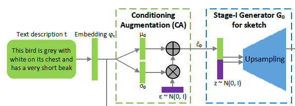
Conditioning Augmentation(CA)

이미지 출처:Stack-GAN

기존에는 text condition을 나타내는 $c$ 를 $\varphi_{t}$ 을 비선형 변환하여 생성했다. 하지만 이런 경우 고정된 $c$ 는 $\varphi_{t}$ 의 높은 차원(100-dimensions 이상)의 latent space를 잘 표현하지 못하고, 데이터의 양이 적을 경우 latent data manifold에 불연속성을 야기한다. 이러한 문제들은 generator 학습에서 바람직하지 못하다.

해당 문제들을 해결하기 위해 Stack-GAN에서 CA를 사용한다. CA는 위의 그림과 같이 $\mu_{0}$ = mean $\mu$ ( $\varphi_{t}$ ), $\sigma_{0}$ = diagonal covariance matrix $\Sigma$ ( $\varphi_{t}$ )를 이용해 $\hat{c}$ 을 $N$ ( $\mu_{0}$ , $\sigma_{0}$ )에서 랜덤 샘플링을 통해 생성한다. 랜덤 샘플링을 위해 표준정규분포에서 랜덤 샘플링한 $\epsilon$ 을 이용해 $\hat{c}$ = $\sigma_{0}$ $\epsilon$ + $\mu_{0}$ 을 구한다.

CA를 통해 coditioning manifold의 작은 변화(perturbation)에 대한 robustness를 증가시킬 수 있다. 또한 CA의 randomness를 통해 text to image translation에서 동일한 text에 대해 다양한 포즈와 형태를 갖는 이미지를 얻을 수 있다.

추가로 conditioning manifold의 smoothness를 강화하고, overfitting을 막기 위해 KL divergence regularization: $D_{KL}(N(\mu(\varphi_{t}),\Sigma(\varphi_{t}))||N(0,I))$ 을 사용한다. 해당 regularization은 generator loss에 추가해서 regularize를 수행한다.
<코드> https://github.com/Maluuba/GeNeVA/blob/master/geneva/definitions/conditioning_augmentor.py

class ConditioningAugmentor(nn.Module):
    def __init__(self, emb_dim, ca_dim):
        super(ConditioningAugmentor, self).__init__()
        self.t_dim = emb_dim
        self.c_dim = ca_dim

        self.fc = nn.Linear(self.t_dim, self.c_dim * 2, bias=True)
        self.relu = nn.ReLU()

    def encode(self, text_embedding):
        x = self.relu(self.fc(text_embedding))
        mu = x[:, :self.c_dim]
        logvar = x[:, self.c_dim:]
        return mu, logvar

    def reparametrize(self, mu, logvar):
        std = logvar.mul(0.5).exp_()
        eps = torch.cuda.FloatTensor(std.size()).normal_()
        return eps.mul(std).add_(mu)

    def forward(self, text_embedding):
        mu, logvar = self.encode(text_embedding)
        c_code = self.reparametrize(mu, logvar)
        return c_code, mu, logvar

Conditional Batch Normalize(CBN)

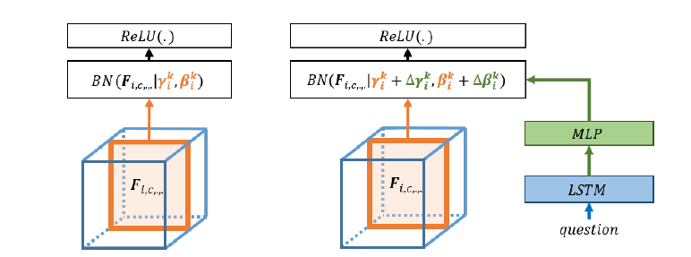
GeNeVA-GAN의 generator의 모든 convolution layer에 CBN을 적용했다.
CBN은 condition에 따라 Batch Normalize(BN)을 적용하는 방법이다.
이미지 출처: Modulating early visual processing by language 논문

기존의 BN에 경우 text embedding 정보를 담고 있는 $\gamma$ , $\beta$ 를 학습하기 여렵다. CBN은 text embedding을 MLP를 통과시킨 값을 기존의 BN에 추가하여 수행한다.

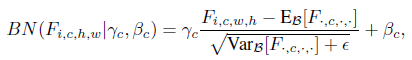
기존의 BN: BN( $F_{i,c,h,w}$ | $\gamma_{c}$ , $\beta_{c}$ )

CBN: BN( $F_{i,c,h,w}$ | $\hat{\gamma_{c}}$ , $\hat{\beta_{c}}$ ), $\hat{\gamma_{c}}$ = $\gamma_{c}$ + $\Delta$ $\gamma_{c}$ , $\hat{\beta_{c}}$ = $\beta_{c}$ + $\Delta$ $\beta_{c}$
$\gamma_{c}$ , $\beta_{c}$ : pre-trained된 값 또는 임의의 초기값
$\Delta$ $\gamma_{c}$ , $\Delta$ $\beta_{c}$ : MLP( $e_{q}$ ), $e_{q}$ = text embedding

CBN의 장점: 컴퓨터 연산적 효율성이 늘어나고, text embedding으로 feature maps를 조작할 수 있게 된다.

<코드> https://github.com/Maluuba/GeNeVA/blob/master/geneva/definitions/conditional_batchnorm.py

class ConditionalBatchNorm2d(nn.Module):
    def __init__(self, in_channels, conditon_dim):
        super().__init__()
        self.channels = in_channels
        self.bn = nn.BatchNorm2d(in_channels, affine=False)
        self.fc = nn.Linear(conditon_dim,
                            in_channels * 2)

        self.fc.weight.data[:, :in_channels] = 1
        self.fc.weight.data[:, in_channels:] = 0

    def forward(self, activations, condition):
        condition = self.fc(condition)
        gamma = condition[:, :self.channels]\
            .unsqueeze(2).unsqueeze(3)
        beta = condition[:, self.channels:]\
            .unsqueeze(2).unsqueeze(3)

        activations = self.bn(activations)
        return activations.mul(gamma).add(beta)

Discriminator part

GeNeVA-GAN은 이미지를 반복적으로 수정하면서 이미지를 생성하므로 각각의 시점에서 이미지의 real/fake 판별로는 충분한 학습이 이루어질 수 없다. 따라서 논문의 저자들은 기존의 discriminator들과 다르게 3가지 변화를 줬다.

image encoder $E_{D}$ 를 이용해 t-1 시점의 ground-truth 이미지 $x_{t-1}$ 과 t시점에 생성된 이미지 $\tilde{x}_{t}$ 를 인코딩 한 후 두 인코딩된 벡터를 fusion layer를 통과시킨다. fusion layer는 학습을 하는 layer가 아닌 인코딩 된 feature map들의 element-wise subtraction 또는 concatation을 수행한다. fusion layer를 이용하는 방법으로 discriminator는 이미지의 변화에 더 집중할 수 있다. 추가로 projection discriminator을 사용했다.
discrminator loss에 real/fake loss외에 (real image, wrong instruction)쌍을 통해 계산되는 wrong loss를 추가했다.
해당 시점에 존재하는 객체(objects)들의 존재를 알기 위한 auxiliary objective를 사용했다.

Projection Discriminator

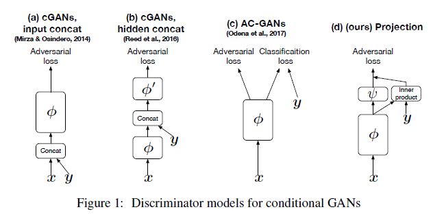이미지 출처: cGANs with Projection Discriminator 논문

f(x,y;\theta) := f_{1}(x,y;\theta) + f_{2}(x;\theta)=y^TV\phi(x;\theta_{\Phi}) + \psi(\phi(x;\theta_{\Phi});\theta_{\Psi})

V: y(condition)에 대한 embedding vector
$\phi$ : 기존의 CNN layers discriminator
$\psi$ : scalar function
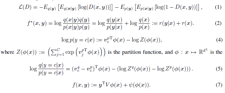이미지 출처: cGANs with Projection Discriminator 논문
p : generated distribution
q : true distribution
r : log likelihood ratio

식(1)의 $D(x,y)$ = $A(f(x,y))$ , A = activation function(주로 sigmoid)
식(2)는 기존의 loss function인 식(1)의 optimal solution $f^*(x,y)$ 을 두 개의 log likelihood ratio의 합으로 나타낸것이다.
log linear model 식(4)를 이용해서 식(2)의 $r(y|x)$ 를 나타낸것이 식(5)이다. 같은 방법으로 식(2)의 $r(x)$ 또한 나타낼 수 있다.
이것들을 정리하면 식(7) $f(x,y)$ 를 정의할 수 있고, 이 식은 위의 식 $f(x,y;\theta)$ 와 같다.

위와 같이 정의된 $f(x,y;\theta)$ 를 이용한 discriminator를 사용하는 경우 기존의 condtional GAN들 보다 성능이 좋았다
<코드>
https://github.com/Maluuba/GeNeVA/blob/master/geneva/models/networks/discriminator_factory.py (코드가 길어서 링크만 첨부)
위 주소의 코드 144~146줄을 보면 projection discriminator의 구현을 확인할 수 있다.

Loss

$c_{t}$ : { $h_{t}$ , $x_{t-1}$ }
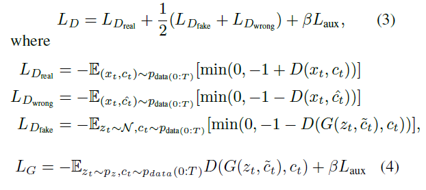
$\hat{c}_{t}$ : t시점의 이미지 $x_{t}$ 와 맞지 않는 instruction
$\tilde{c}_{t}$ : { $h_{t}$ , $f_{G_{t-1}}$ }
Hinge Advesarial Loss를 사용했다.

Hinge Adversarial Loss

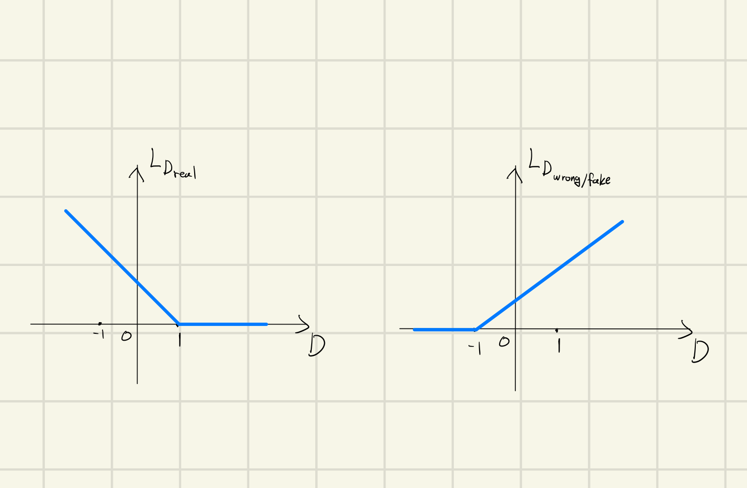
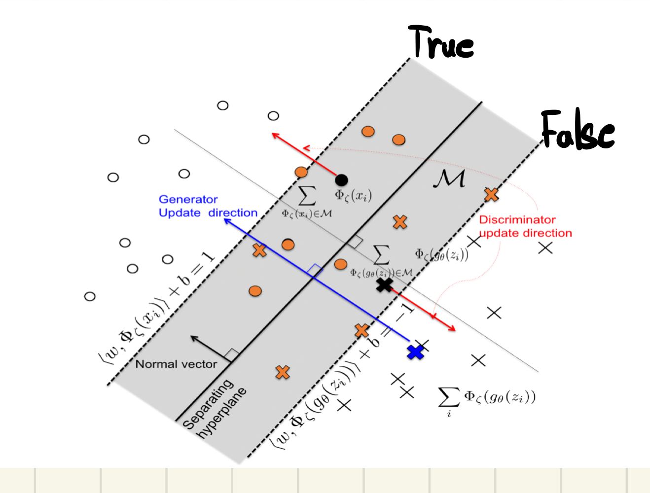
이미지 출처: Geometric-GAN

Discriminator의 마지막 활성화 함수는 identity function으로 sigmoid를 사용하지 않는다. real pair ( $x_{t}$ , $c_{t}$ )에 대해 discriminator 출력값이 1 이하인 경우에만 학습하고, fake/wrong pair에 대해 discriminator 출력값이 -1이상인 경우에만 학습을 한다.
hinge loss를 사용하면 기존의 gan loss보다 mode collapse 문제를 해결할 수 있다는 장점이 있다.
<코드> https://github.com/Maluuba/GeNeVA/blob/master/geneva/criticism/losses.py

class HingeAdversarial():
    @staticmethod
    def discriminator(real, fake, wrong=None, wrong_weight=0.):

        l_real = F.relu(1. - real).mean()
        l_fake = F.relu(1. + fake).mean()

        if wrong is None:
            return l_real + l_fake
        else:
            l_wrong = F.relu(1. + wrong).mean()
            return l_real + wrong_weight * l_wrong + (1. - wrong_weight) * l_fake

Auxiliary Loss

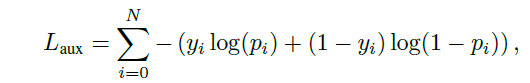
t 시점 N개(dataset에 존재하는 모든 개체의 수)의 개체 각각에 대한 BCEloss를 계산한다. 뒤에 설명할 projection conditioning 이전의 discriminator layer에 N차원 linear layer를 추가하고, 활성화 함수로 sigmoid를 사용하여 각각의 $p_{i}$ 를 얻는다.

Zero-centered Gradient Panalty

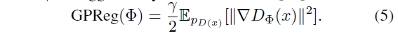
학습의 안정성을 위해 discriminator의 parameters $\Phi$ 를 regularize 시킨다. gradient가 커지는 것을 막아준다. ( $\gamma$ :hyper parameter)

Implementation Details

model의 구조와 관련된 2가지

self-attention layer
spectral normalization

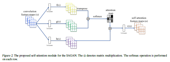
Self-Attention Layer

GeNeVA-GAN의 generator/discriminator의 layers 중간에 들어간다.

Self-Attention GAN(SAGAN)은 기존의 convolutional 연산만을 이용한 GAN은 CNN의 local receptive field로 인하여 Long-range dependence를 잘 고려하지 못하는 문제를 해결하기 위해 self-attention을 적용했다.

참고) Long-range dependence(LRD): is a phenomenon that may arise in the analysis of spatial or time series data. It relates to the rate of decay of statistical dependence of two points with increasing time interval or spatial dsitance between the points => 시간 간격/공간 거리가 증가함에 따라 두점의 통계적 의존성 붕괴율과 관련됨
이미지 출처: SA-GAN 논문

<코드>https://github.com/Maluuba/GeNeVA/blob/master/geneva/definitions/self_attention.py

class SelfAttention(nn.Module):
    def __init__(self, C):
        super(SelfAttention, self).__init__()

        self.f_x = spectral_norm(
            nn.Conv2d(in_channels=C, out_channels=C // 8, kernel_size=1))
        self.g_x = spectral_norm(
            nn.Conv2d(in_channels=C, out_channels=C // 8, kernel_size=1))
        self.h_x = spectral_norm(
            nn.Conv2d(in_channels=C, out_channels=C, kernel_size=1))

        self.gamma = nn.Parameter(torch.zeros(1))

    def forward(self, x):
        B, C, H, W = x.size()
        N = H * W

        f = self.f_x(x).view(B, C // 8, N)
        g = self.g_x(x).view(B, C // 8, N)

        s = torch.bmm(f.permute(0, 2, 1), g)  # f(x)^{T} * g(x)
        beta = F.softmax(s, dim=1)

        h = self.h_x(x).view(B, C, N)
        o = torch.bmm(h, beta).view(B, C, H, W)

        y = self.gamma * o + x

        return y

Spectoral Normalization(SN)

GeNeVA-GAN의 discriminator의 모든 layer에 SN을 사용했다. SN은 다른 normalize와 같이 pytorch에 구현되있다.
이미지 출처: SN-GAN

$D(x,\theta)$ = $A(f(x,\theta))$ , A: activation function
$\nabla f$ 가 유계가 아니거나 심지어 계산이 불가능할 수 있다. 이러한 문제를 해결하기 위해 $||f||_{Lip} \le K$ 즉 K-Lipschitz 제약을 준다.
$||f||_{Lip} \le M$ 은 $L_{2}$ norm을 이용해 정해진 구간에서 임의의 $x$ , $x'$ 에 대해 $||f(x) - f(x')|| / ||x-x'||$ $\le$ M을 의미한다. 여기서 M은 립시츠 상수

이와 같은 립시츠 제약은 WGAN에서 사용되었다. WGAN은 1-립시츠 제약을 위해 weight clipping을 사용했었다.
이미지 출처: SN-GAN

$\sigma$ : spectral norm( $L_{2}$ matrix norm)
$\sigma(A)$ : $A^T$ $A$ 의 eigen value 중 가장 큰 값을 $\lambda_{1}$ 일 때, $\sqrt{\lambda_{1}}$

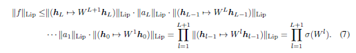
식(7)을 보면 $||f||_{Lip}$ 의 립시츠 상수는 각 layer의 W들의 spectral norm의 곱들보다 작다. 따라서 각 layer의 W를 $\sigma$ (W)로 normalize 하면 즉 W = $W/\sigma(W)$ 이면 립시츠 상수가 1이 된다.

SN은 각 layer의 transformation이 한 방향으로 민감(sensitive)해지는 것을 방지한다. 이러한 원리로 SN-GAN은 WGAN, WGAN-GP, Batch Norm, Layer Norm 등의 다른 방법들 보다 좋은 성능을 보였다.

Evaluation

성능 평가를 위해 Inception-v3 구조를 기반으로 한 object detector와 localizer를 만들었다. Inception-v3의 마지막 layer를 linear layer with sigmoid와 linear layer 두 부분으로 수정하여 첫 번째 부분은 object detect를 위한 분류기로 사용하고, 두 번째 부분은 localizer를 위해 개체의 좌표를 회귀한다.

GeNeVA-GAN의 성능평가는 기존의 GAN의 성능평가를 위한 Inception score와 FID가 부적절하여 object detecotor와 localizer를 이용해 precision,recall,F1-score를 구한다. 또한 object detector와localizer를 이용해 노드가 개체이고, 엣지가 위치관계(앞,뒤,좌,우)인 그래프를 생성한다. real/fake 이미지의 그래프를 비교해 개체들이 올바른 위치에 존재하는지 평가할 수 있다. 이 평가를 위해 Relational Similarity를 구한다.

Relational Similarity

관계 유사성으로 개체가 올바른 위치에 있는지 평가한다.

rsim(E_{G_{gt}},E_{G_{gen}}) = recall * \frac {\vert E_{G_{gen}} \cap E_{G_{gt}}\vert} {\vert E_{G_{gt}}|}

real/fake 이미지가 같은 개체들을 갖고 있는 경우 중 위치가 일치하는 비율에 recall을 곱해서 Relational Similarity를 구할 수 있다.

<코드> https://github.com/Maluuba/GeNeVA/blob/master/geneva/metrics/inception_localizer.py

def get_graph_similarity(detections, label, locations, gt_locations, dataset):
    intersection = (detections & label).astype(bool)
    if not np.any(intersection):
        return 0

    locations = locations.data.cpu().numpy()[intersection]
    gt_locations = gt_locations.data.cpu().numpy()[intersection]

    genereated_graph = construct_graph(locations, dataset)
    gt_graph = construct_graph(gt_locations, dataset)

    matches = (genereated_graph == gt_graph).astype(int).flatten()
    matches_accuracy = matches.sum() / len(matches)
    recall = recall_score(label, detections, average='samples')

    graph_similarity = recall * matches_accuracy

    return graph_similarity

Conclusion

GeNeVA-GAN을 통해 주어진 instructions에 따라 반복적으로 합리적인 그림을 그릴 수 있는 것을 확인했다. 실험을 통해 비반복적 방법도 어느 정도 성능을 보일 수 있으나 반복적인 방법에 비해 낮은 성능을 확인했다. 또한 해당 모델을 위한 새로운 metric(Relational Similarity)을 제안했다.
마지막으로 실제 사진과 같은 이미지로 학습하기 위해 해당 모델에 맞는 주석이 달려있는 image sequence가 필요하다.

References

Geometric-GAN: Jae Hyun Lim and Jong Chul Ye, “Geometric GAN,”
arXiv:1705.02894 [stat.ML], 2017.

SN-GAN: Takeru Miyato, Toshiki Kataoka, Masanori Koyama,
and Yuichi Yoshida, “Spectral normalization for generative
adversarial networks,” in International Conference
on Learning Representations (ICLR), 2018.

SA-GAN: Han Zhang, Ian Goodfellow, Dimitris Metaxas, and
Augustus Odena, “Self-attention generative adversarial
networks,” arXiv:1805.08318 [stat.ML], 2018.

projection discriminator: Takeru Miyato and Masanori Koyama, “cGANs with
projection discriminator,” in International Conference
on Learning Representations (ICLR), 2018.

zero-gentered gradient penalty: Lars Mescheder, Andreas Geiger, and Sebastian
Nowozin, “Which training methods for GANs do actually
converge?” in International Conference on Machine
learning (ICML), 2018.

conditional batch normalization: Harm de Vries, Florian Strub, J´er´emie Mary, Hugo Larochelle, Olivier Pietquin, and Aaron C Courville. Modulating
early visual processing by language. In NIPS, pp. 6576–6586, 2017.

Stack-GAN: Han Zhang, Tao Xu, Hongsheng Li, Shaoting Zhang,
Xiaogang Wang, Xiaolei Huang, and Dimitris N.
Metaxas, “StackGAN: Text to photo-realistic image
synthesis with stacked generative adversarial networks,”
in International Conference on Computer Vision
(ICCV), 2017.

출처가 없는 이미지: GeNeVA-GAN 논문 내의 이미지

김상현

Mucha Suerte

이전 포스트

Build Better Generative Adversarial Networks

다음 포스트