CNN 33 - CNN 필터 시각화

1. MNIST 데이터 세트에 대한 기본 CNN 교육, Keras

2. 필터 시각화

3. 입력 영상을 전파할 때 필터 활성화를 시각화합니다

MNIST Dataset로 기본적인 CNN 모델 Training

# TensorFlow에서 내장된 데이터셋을 불러옵니다
from tensorflow.keras.datasets import mnist

# MNIST 훈련 및 테스트 데이터셋을 로드합니다
(x_train, y_train), (x_test, y_test) = mnist.load_data()

# GPU를 사용하고 있는지 확인합니다
from tensorflow.python.client import device_lib

print(device_lib.list_local_devices())

# x_train, x_test, y_train, y_test의 샘플 수를 출력합니다
print("x_train의 초기 모양 또는 차원: ", str(x_train.shape))

# 데이터 샘플 수를 출력합니다
print("훈련 데이터의 샘플 수: " + str(len(x_train)))
print("훈련 데이터의 레이블 수: " + str(len(y_train)))
print("테스트 데이터의 샘플 수: " + str(len(x_test)))
print("테스트 데이터의 레이블 수: " + str(len(y_test)))

# 훈련 및 테스트 데이터의 이미지 차원과 레이블 수를 출력합니다
print("\n")
print("x_train의 차원: " + str(x_train[0].shape))
print("x_train의 레이블: " + str(y_train.shape))
print("\n")
print("x_test의 차원: " + str(x_test[0].shape))
print("y_test의 레이블: " + str(y_test.shape))

코드를 여러개 나눠서 말고 한번에 실행

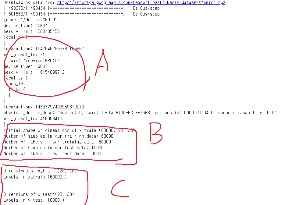
A : GPU 사용중인지 확인 - CUDA 이용해 학습 위함
B : Train, Test 데이터 셋 갯수와, 형태 확인 - 28x28 그레이스케일
C : Dimensions(차원), Labels(레이블)

Keras 형태에 맞게 데이터셋에 차원 추가, 정규화 및 원-핫 인코딩

# 행과 열의 수를 저장합니다
img_rows = x_train[0].shape[0]
img_cols = x_train[0].shape[1]

# Keras에서 필요한 '형태'로 데이터를 맞추기
# 데이터에 4번째 차원을 추가하여
# 원래 이미지 형태 (60000,28,28)를 (60000,28,28,1)로 변경합니다
x_train = x_train.reshape(x_train.shape[0], img_rows, img_cols, 1)
x_test = x_test.reshape(x_test.shape[0], img_rows, img_cols, 1)

# 단일 이미지의 형태를 저장합니다
input_shape = (img_rows, img_cols, 1)

# 이미지 타입을 float32 데이터 타입으로 변경합니다
x_train = x_train.astype('float32') # 원래는 uint8
x_test = x_test.astype('float32')

# 데이터 범위를 (0에서 255)에서 (0에서 1)로 변경하여 정규화합니다
x_train /= 255.0
x_test /= 255.0

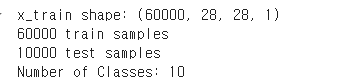
print('x_train shape:', x_train.shape)
print(x_train.shape[0], 'train samples')
print(x_test.shape[0], 'test samples')

from tensorflow.keras.utils import to_categorical

# 출력을 원-핫 인코딩합니다
y_train = to_categorical(y_train)
y_test = to_categorical(y_test)

# 원-핫 인코딩된 행렬의 열 수를 셉니다
print("Number of Classes: " + str(y_test.shape[1]))

num_classes = y_test.shape[1]
num_pixels = x_train.shape[1] * x_train.shape[2]

Keras 모델 빌드

from tensorflow.keras.models import Sequential
from tensorflow.keras.layers import Dense, Dropout, Flatten
from tensorflow.keras.layers import Conv2D, MaxPooling2D
from tensorflow.keras import backend as K
from tensorflow.keras.optimizers import SGD 

model = Sequential()
model.add(Conv2D(32, kernel_size=(3, 3), activation='relu', input_shape=input_shape))
model.add(Conv2D(64, (3, 3), activation='relu'))
model.add(MaxPooling2D(pool_size=(2, 2)))
model.add(Flatten())
model.add(Dense(128, activation='relu'))
model.add(Dense(num_classes, activation='softmax'))

model.compile(loss = 'categorical_crossentropy',
              optimizer = SGD(0.001),
              metrics = ['accuracy'])

print(model.summary())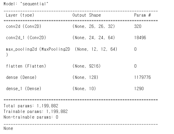

Dense = FC1,
Dense_1 = FC2 = Softmax

모델 트레이닝, 에포크 10

batch_size = 128
epochs = 10

# 결과를 저장하여 나중에 플롯팅할 수 있도록 합니다
# fit 함수에서 데이터셋(x_train 및 y_train), 배치 크기(보통 16에서 128, RAM에 따라 다름),
# 에포크 수(보통 10에서 100) 및 검증 데이터셋(x_test 및 y_test)을 지정합니다
# verbose = 1은 매 에포크마다 성능 지표를 출력하도록 설정합니다
history = model.fit(x_train,
                    y_train,
                    batch_size=batch_size,
                    epochs=epochs,
                    verbose=1,
                    validation_data=(x_test, y_test))

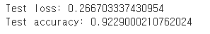
# evalute 함수를 사용하여 정확도 점수를 얻습니다
# score는 테스트 손실과 정확도의 두 값을 가집니다
score = model.evaluate(x_test, y_test, verbose=0)
print('Test loss:', score[0])
print('Test accuracy:', score[1])

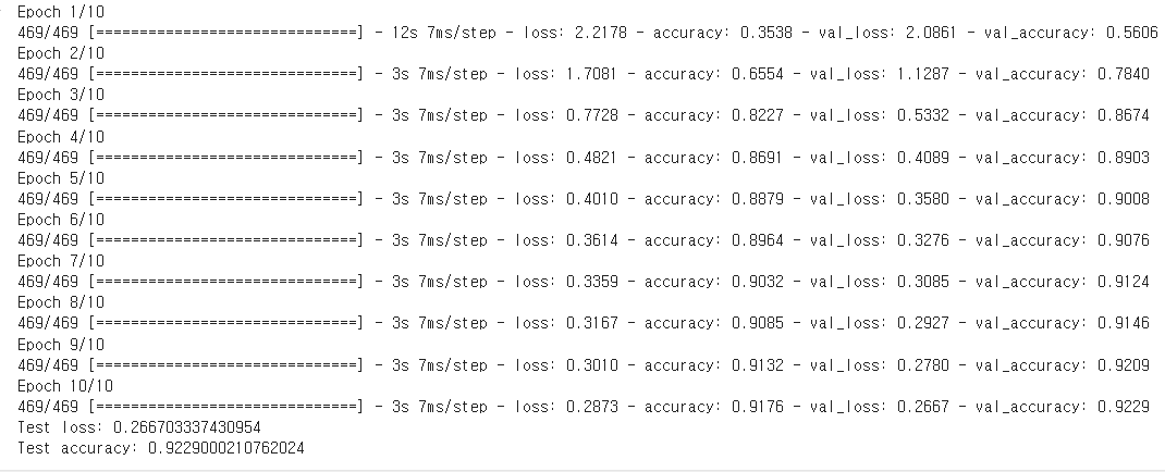
10회의 트레이닝 모델을

x_test, y_test, 즉 테스트 데이터셋(10000,28,28,1)을 이용해서 검증한 결과

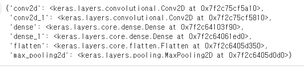
Key Layer의 Symbolic Output 얻기

# 모델의 각 레이어의 이름과 해당 레이어 객체를 딕셔너리로 만듭니다
layer_dict = dict([(layer.name, layer) for layer in model.layers])
layer_dict

model.layers 는 모델에 있는 모든 레이어의 리스트를 제공

리스트 내포를 사용하여 각 레이어의 이름(layer.name)과 레이어 객체(layer)를 쌍으로 묶어 딕셔너리를 만든다.

6개의 레이어에 대해 딕셔너리를 생성한 결과

Conv 필터의 모양만 가져오기

# 필터 형태 요약하기
for layer in model.layers:
  # 합성곱 레이어인지 확인합니다
  if 'conv' not in layer.name:
    continue

  # 필터 가중치 가져오기
  filters, biases = layer.get_weights()
  print(layer.name, filters.shape)

1. for layer in model.layers:
   model.layers 리스트를 순회하여 각 레이어를 확인
2. 합성곱(Conv) 레이어 인지 확인

if 'conv' not in layer.name:
  continue

레이어 이름에 conv가 포함되어 있지 않으면 다음 레이어로 넘어감
3. 필터 가중치 가졍오기

filters, biases = layer.get_weights()
print(layer.name, filters.shape)

layer.get_weights()를 사용하여 레이어의 가중치(필터와 바이어스)를 가져온다.

결과

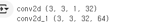
아까 모델 빌드하고 출력한 model.summary()와 비교해보면

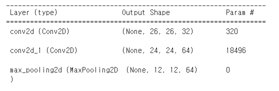
Conv_1(conv2d) 는 32개의 필터와 각 필터는 3x3 크기이며, 입력 채 널 수는 1
Conv_2(conv2d_1) 은 3x3 필터가 64개 있고, 32개의 차원으로 돼있다.

첫 번째 Conv Layer의 무게 확인

1. 첫 번째 합성곱 레이어에서 가중치 가져오기:

# 첫 번째 합성곱(은닉) 레이어에서 가중치를 가져옵니다
filters, biases = model.layers[0].get_weights()

2. 필터 확인:

3x3 필터 크기, 1채널 수, 32 필터의 수

즉, 이 레이어는 32개의 서로 다른 3x3 필터를 사용

# 필터를 확인해봅니다
print(filters.shape)
filters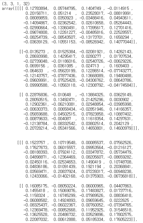

3. 바이어스 확인:

# 이제 바이어스를 확인해봅니다
print(biases.shape)
biases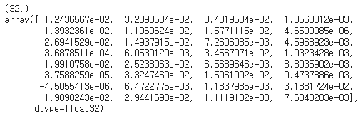

(32, ) 는 바이어스의 형태이고,

이는 각 필터에 하나의 바이어스 값이 있음을 나타낸다.

필터와 바이어스의 역할

필터:
각 필터는 입력 이미지의 특정 부분을 인식하고, 이를 통해 이미지의 특징을 추출
필터의 값들은 학습 과정에서 조정

바이어스:
필터의 출력에 더해져서 필터가 특정 특징을 더 잘 인식할 수 있도록 도와준다.

필터 값을 0-1로 정규화하여 시각화

필터 가중치 범위를 정규화해서 이해하기 힘든 전의 데이터를 이해하기

쉬운 값으로 변경한다.

# 필터 값을 0-1로 정규화하여 시각화합니다
f_min, f_max = filters.min(), filters.max()
#최댓값 최소값 출력
print(f'Before Normalisation, Min = {f_min} and Max =  {f_max}')
filters = (filters - f_min) / (f_max - f_min)
print(f'After Normalisation, Min = {filters.min()} and Max =  {filters.max()}')

위의 출력이 무슨 말인지 보자.
아래는 필터의 값을 출력했던것인데,

저 값에서 가장 최소값을 0 으로 최댓값을 1로 기준으로 잡아서

정규화를 한것이고,

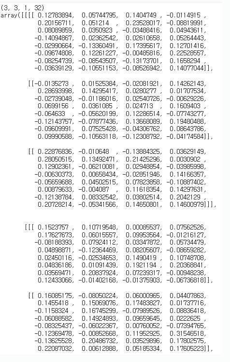
정규화 전의 최댓값, 최소값을 출력해준것.

필터 값의 최소값: -0.14094866812229156
필터 값의 최대값: 0.31546518206596375

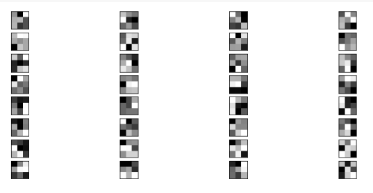
학습된 필터 시각화

값으로만 본 필터를 이제 시각화 해보자.

import matplotlib.pyplot as plt
import numpy as np

# 첫 번째 몇 개의 필터를 시각화하고 플롯 크기를 설정합니다
n_filters, ix = 32, 1
plt.figure(figsize=(12,20))

for i in range(n_filters):
    # 필터를 가져옵니다
    f = filters[:, :, :, i]
    #print(f.shape)

    # 4 x 8 서브플롯으로 배열합니다
    ax = plt.subplot(n_filters, 4, ix)
    ax.set_xticks([])
    ax.set_yticks([])

    # 필터 채널을 회색조로 플롯합니다
    plt.imshow(np.squeeze(f, axis=2), cmap='gray')
    ix += 1
    
# 플롯을 표시합니다
plt.show()

필터를 4x8 서브플롯으로 배열하고, 각 필터 채널을 그레이스케일로 표현

상위 2개의 레이어 출력 추출 및 시각화

1. 상위 2개의 레이어 출력 추출 & 출력 모델 생성:

from tensorflow.keras.models import Model

# 상위 2개의 레이어 출력을 추출합니다
layer_outputs = [layer.output for layer in model.layers[:2]]

# 모델 입력을 주면 이 출력들을 반환하는 모델을 생성합니다
activation_model = Model(inputs=model.input, outputs=layer_outputs)

layer_outputs

모델 레이어에서 첫 두 레이러를 가져오면

Conv_1 , Conv_2가 가져와진다.

그 두개의 모델을 받기위한 Model을 생성 > activation_model

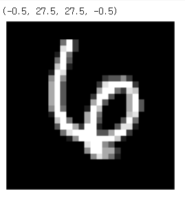
2. 테스트 이미지 시각화:

import matplotlib.pyplot as plt

# 테스트 세트의 22번째 이미지를 가져와서 형태를 (1, 28, 28, 1)로 재조정합니다
img_tensor = x_test[22].reshape(1,28,28,1)

# 이미지를 시각화합니다
fig = plt.figure(figsize=(5,5))
plt.imshow(img_tensor[0,:,:,0], cmap="gray")
plt.axis('off')

테스트 데이터셋의 22번째 이미지를 가져와서

형태를 재조정한다음 이미지를 시각화 했다.

(-0.5, 27.5, 27.5, -0.5)이 값은 이미지의 픽셀 좌표를 나타낸다.

x(-0.5~27.5), y(-0.5~27.5) 이 범위는 이미지가 28x28 픽셀 크기임을 나타낸다.

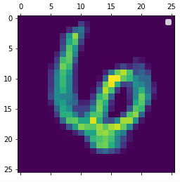
첫 번째 합성곱 레이어의 네 번째 필터 출력 시각화

첫 번째 합성곱 레이어의 네 번째 필터 출력을 시각화하여, 모델이 입력 이미지에서 학습한 특정 특징을 어떻게 추출하는지 확인한다.

import matplotlib.pyplot as plt

# 첫 번째 합성곱 레이어의 네 번째 필터 출력 시각화
plt.matshow(first_layer_activation[0, :, :, 3], cmap='viridis')
plt.title("4th Filter Feature Map in 1st Conv Layer")
plt.axis('off')
plt.show()

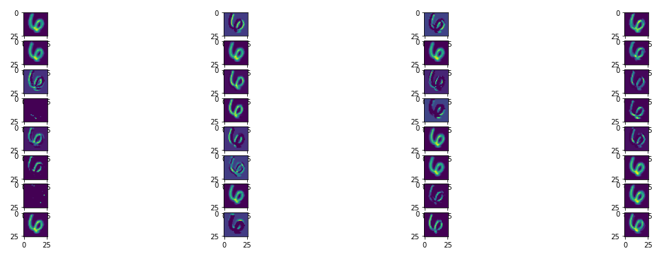
활성화 맵 시각화 함수 (Activation Map Visualization Function)

모델의 특정 레이어에서 계산된 활성화 맵을 시각화하여, 각 필터가 입력 데이터에서 학습한 특징을 어떻게 추출되는지 확인

import matplotlib.pyplot as plt

def display_activation(activations, col_size, row_size, act_index): 
    # 주어진 인덱스의 활성화 맵을 가져옵니다
    activation = activations[act_index]
    activation_index = 0
    
    # 행(row_size)과 열(col_size) 크기로 서브플롯을 생성합니다
    fig, ax = plt.subplots(row_size, col_size, figsize=(row_size*2.5, col_size*1.5))
    
    # 각 서브플롯에 활성화 맵의 필터 출력을 시각화합니다
    for row in range(row_size):
        for col in range(col_size):
            # 현재 활성화 맵의 특정 필터 출력을 시각화합니다
            ax[row][col].imshow(activation[0, :, :, activation_index], cmap='viridis')
            activation_index += 1

    # 플롯 사이의 간격을 조정하여 더 깔끔하게 만듭니다
    plt.tight_layout()
    plt.show()

4x8 격자 맵을 만들어 첫번째 Conv_1 레이어의 32개의 필터 활성화 맵을 시각화 한다.