앞 초기 설정 부분은 저번 내용과 똑같다.
정규화를 적용한 CNN 구축
드롭아웃(Dropout) 추가
컨볼루션 신경망(CNN)에서는 드롭아웃을 주로 CONV-RELU 층 뒤에 추가
예시: CONV -> RELU -> DROPOUT
비율은 0.1~0.3 사이의 값이 잘 작동하고, 0.2를 사용할 것이다.
배치 정규화(BatchNorm) 추가
CNN에서 BatchNorm은 컨볼루션 층과 활성화 함수 층(ReLU) 사이에 사용하는 것이 가장 좋다.
CONV_1 -> BatchNorm -> ReLU -> Dropout -> CONV_2
import torch.nn as nn
import torch.nn.functional as F
# 신경망 클래스 정의
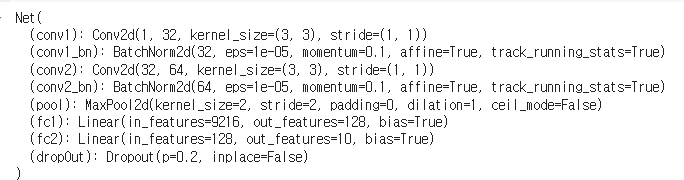
class Net(nn.Module):
def __init__(self):
super(Net, self).__init__()
# 첫 번째 컨볼루션 층: 입력 채널 1, 출력 채널 32, 커널 크기 3x3
self.conv1 = nn.Conv2d(1, 32, 3)
# 배치 정규화 추가, 입력으로 32 사용 (첫 번째 컨볼루션 층의 출력)
self.conv1_bn = nn.BatchNorm2d(32)
# 두 번째 컨볼루션 층: 입력 채널 32, 출력 채널 64, 커널 크기 3x3
self.conv2 = nn.Conv2d(32, 64, 3)
#### 배치 정규화 추가, 입력으로 64 사용 (두 번째 컨볼루션 층의 출력)
self.conv2_bn = nn.BatchNorm2d(64)
# 최대 풀링 층: 커널 크기 2x2
self.pool = nn.MaxPool2d(2, 2)
# 첫 번째 완전 연결 층: 입력 크기 64 * 12 * 12, 출력 크기 128
self.fc1 = nn.Linear(64 * 12 * 12, 128)
# 두 번째 완전 연결 층: 입력 크기 128, 출력 크기 10 (클래스 개수)
self.fc2 = nn.Linear(128, 10)
# 드롭아웃 함수 정의, 비율 0.2
self.dropOut = nn.Dropout(0.2)
def forward(self, x):
# 첫 번째 컨볼루션, 배치 정규화, ReLU, 드롭아웃 적용
x = F.relu(self.conv1_bn(self.conv1(x)))
x = self.dropOut(x)
# 두 번째 컨볼루션, 배치 정규화, ReLU, 드롭아웃 적용
x = self.dropOut(F.relu(self.conv2_bn(self.conv2(x))))
# 최대 풀링 적용
x = self.pool(x)
# 특성 맵을 일렬로 펼침
x = x.view(-1, 64 * 12 * 12)
# 첫 번째 완전 연결 층과 ReLU 적용
x = F.relu(self.fc1(x))
# 두 번째 완전 연결 층 적용 (출력)
x = self.fc2(x)
return x
# 신경망 인스턴스 생성 및 장치로 이동 (GPU 또는 CPU)
net = Net()
net.to(device)
L2 정규화 추가
# 옵티마이저 함수 불러오기
import torch.optim as optim

# 교차 엔트로피 손실 함수를 손실 함수로 사용
criterion = nn.CrossEntropyLoss()

# 경사 하강법 알고리즘 또는 옵티마이저 설정
# 학습률 0.001로 설정된 확률적 경사 하강법(SGD)을 사용
# 모멘텀(momentum)을 0.9로 설정, weight_decay를 0.001로 설정하여 L2 정규화 적용
optimizer = optim.SGD(net.parameters(), lr=0.001, momentum=0.9, weight_decay=0.001)
L2 값은 0.001을 사용했다.
데이터 증강, 드롭아웃, 배치 규범 및 L2 정규화를 사용한 모델 학습
# 훈련 데이터셋을 여러 번 반복 (각 반복은 에폭(epoch)이라고 함)
epochs = 15
# 로그를 저장할 빈 배열 생성
epoch_log = []
loss_log = []
accuracy_log = []
# 지정된 에폭 수 만큼 반복
for epoch in range(epochs):
print(f'Starting Epoch: {epoch+1}...')
# 각 미니 배치 후 손실을 누적하여 저장
running_loss = 0.0
# trainloader 이터레이터를 통해 반복
# 각 사이클은 미니 배치
for i, data in enumerate(trainloader, 0):
# 입력과 레이블 가져오기; data는 [inputs, labels] 리스트
inputs, labels = data
# 데이터를 GPU로 이동
inputs = inputs.to(device)
labels = labels.to(device)
# 학습 전 기울기 초기화 (0으로 설정)
optimizer.zero_grad()
# 순전파 -> 역전파 + 최적화
outputs = net(inputs) # 순전파
loss = criterion(outputs, labels) # 손실 계산 (예측 결과와 실제 값의 차이)
loss.backward() # 역전파를 통해 모든 노드의 새로운 기울기 계산
optimizer.step() # 기울기/가중치 업데이트
# 학습 통계 출력 - 에폭/반복/손실/정확도
running_loss += loss.item()
if i % 100 == 99: # 100 미니 배치마다 손실 출력
correct = 0 # 올바른 예측 개수를 저장할 변수 초기화
total = 0 # 반복된 레이블의 총 개수를 저장할 변수 초기화
# 검증 과정에서는 기울기가 필요 없으므로
# no_grad로 감싸서 메모리 절약
with torch.no_grad():
# testloader 이터레이터를 통해 반복
for data in testloader:
images, labels = data
# 데이터를 GPU로 이동
images = images.to(device)
labels = labels.to(device)
# 테스트 데이터 배치를 모델에 통과시키기 (순전파)
outputs = net(images)
# 최대값에서 예측값 가져오기
_, predicted = torch.max(outputs.data, 1)
# 총 레이블 개수를 total 변수에 계속 추가
total += labels.size(0)
# 올바르게 예측된 개수를 correct 변수에 계속 추가
correct += (predicted == labels).sum().item()
accuracy = 100 * correct / total
epoch_num = epoch + 1
actual_loss = running_loss / 100
print(f'Epoch: {epoch_num}, Mini-Batches Completed: {(i+1)}, Loss: {actual_loss:.3f}, Test Accuracy = {accuracy:.3f}%')
running_loss = 0.0
# 각 에폭 후 학습 통계 저장
epoch_log.append(epoch_num)
loss_log.append(actual_loss)
accuracy_log.append(accuracy)
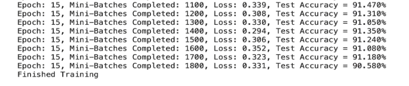
print('Finished Training')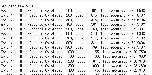
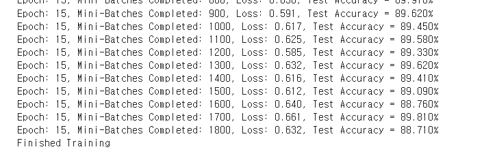
정규화 적용안하고 학습한 정확도
Keras에서 확인했던것처럼
에포크가 적은 경우 비정규화의 정확도가 더 높다.
25~50회 정도 학습을 할 경우 높은 경우를 갖는데,
정규화의 특징 중에 학습수가 적을경우
오히려 정확도가 떨어질수 있다는 특징이 있으므로 각 프로젝트
목적에 맞춰서 확인을 해야한다.
정확도 확인
correct = 0
total = 0

with torch.no_grad():
    for data in testloader:
        images, labels = data
        # Move our data to GPU
        images = images.to(device)
        labels = labels.to(device)
        outputs = net(images)
        _, predicted = torch.max(outputs.data, 1)
        total += labels.size(0)
        correct += (predicted == labels).sum().item()

accuracy = 100 * correct / total
print(f'Accuracy of the network on the 10000 test images: {accuracy:.4}%')
시간에 따른 값 확인
# 최종 테스트 데이터에 대한 정확도 계산
correct = 0
total = 0

with torch.no_grad():
    for data in testloader:
        images, labels = data
        # 데이터를 GPU로 이동
        images = images.to(device)
        labels = labels.to(device)
        outputs = net(images)
        _, predicted = torch.max(outputs.data, 1)
        total += labels.size(0)
        correct += (predicted == labels).sum().item()

accuracy = 100 * correct / total
print(f'Accuracy of the network on the 10000 test images: {accuracy:.4}%')

# 결과 시각화
import matplotlib.pyplot as plt

# 보조 y축이 있는 플롯을 생성하기 위해 서브플롯 생성
fig, ax1 = plt.subplots()

# 제목과 x축 레이블 회전 설정
plt.title("Accuracy & Loss vs Epoch Mini-Batches")
plt.xticks(rotation=45)

# 보조 y축을 생성하기 위해 twinx 사용
ax2 = ax1.twinx()

# loss_log와 accuracy_log를 플롯
ax1.plot(epoch_log, loss_log, 'g-')
ax2.plot(epoch_log, accuracy_log, 'b-')

# 레이블 설정
ax1.set_xlabel('Epochs')
ax1.set_ylabel('Loss', color='g')
ax2.set_ylabel('Test Accuracy', color='b')

plt.show()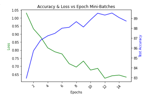

감사합니다. https://www.youtube.com/channel/UCxlkiu9_aWijoD7BannNM7w