목표
1. Houghlines
2. Probabilistic Houghlines
3. Hough Circles
4. Blob Detection
1. Houghlines
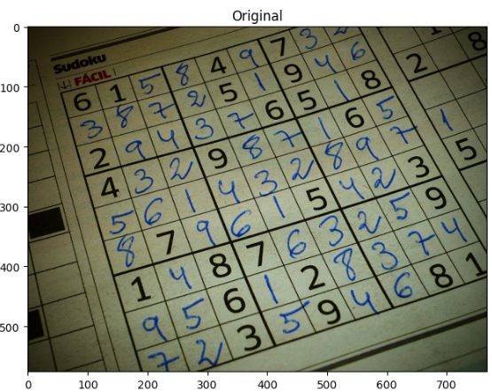
image = cv2.imread('images/soduku.jpg')
imshow('Original', image)
# Grayscale and Canny Edges extracted
gray = cv2.cvtColor(image, cv2.COLOR_BGR2GRAY)
edges = cv2.Canny(gray, 100, 170, apertureSize = 3)
# Run HoughLines using a rho accuracy of 1 pixel
# theta accuracy of np.pi / 180 which is 1 degree
# Our line threshold is set to 240 (number of points on line)
lines = cv2.HoughLines(edges, 1, np.pi / 180, 240)
# We iterate through each line and convert it to the format
# required by cv2.lines (i.e. requiring end points)
for line in lines:
rho, theta = line[0]
a = np.cos(theta)
b = np.sin(theta)
x0 = a * rho
y0 = b * rho
x1 = int(x0 + 1000 * (-b))
y1 = int(y0 + 1000 * (a))
x2 = int(x0 - 1000 * (-b))
y2 = int(y0 - 1000 * (a))
cv2.line(image, (x1, y1), (x2, y2), (255, 0, 0), 2)
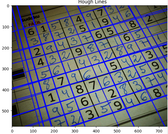
imshow('Hough Lines', image)이 코드는 이미지에서 직선을 검출하는 Hough 변환을 수행
- 그레이스케일 및 엣지 검출:
- 주어진 이미지를 그레이스케일로 변환하고, Canny 엣지 검출을 사용하여 엣지를 추출
이 단계에서는 이미지에서 주요한 선들을 찾기 위해 엣지를 추출하는데 사용
- Hough 변환 실행:
- cv2.HoughLines 함수를 사용하여 Hough 변환을 실행합니다. 이 함수는 직선을 감지하고 직선의 파라미터를 반환합니다.
- 함수에 전달되는 매개변수는 다음과 같습니다:
- edges: 엣지 이미지
- rho : Hough 변환에서 rho 값의 정확도(단위 : 1px)
- theta : Hough 변환에서 theta 값(각도)의 정확도
- threshold : 선으로 인정되기 위한 엣지 점의 최소 수(값이 높을수록 인식되는 선의 수가 줄어듬)
Original Image
Hough Lines
2. Probabilistic Houghlines
확률적 Houghlines
일반적인 Houghline 방식이 있는데 확률적 Houghlines이 왜 개발이 됐을까?
동작에는 이상이 없지만 기존의 방식은 컴퓨터 비용이 많이들어갔다.
그래서 복잡성을 줄이기 위해 확률적 Houghlines 쪽으로 자연스레 개발이 됐다.
코드도 기존의 방식보다 확실히 짧다.
# Grayscale and Canny Edges extracted
image = cv2.imread('images/soduku.jpg')
gray = cv2.cvtColor(image, cv2.COLOR_BGR2GRAY)
edges = cv2.Canny(gray, 100, 170, apertureSize = 3)

# Again we use the same rho and theta accuracies
# However, we specific a minimum vote (pts along line) of 100
# and Min line length of 3 pixels and max gap between lines of 25 pixels
lines = cv2.HoughLinesP(edges, 1, np.pi / 180, 100, 3, 25)
print(lines.shape)

for x in range(0, len(lines)):
    for x1,y1,x2,y2 in lines[x]:
        cv2.line(image,(x1,y1),(x2,y2),(0,255,0),2)

imshow('Probabilistic Hough Lines', image)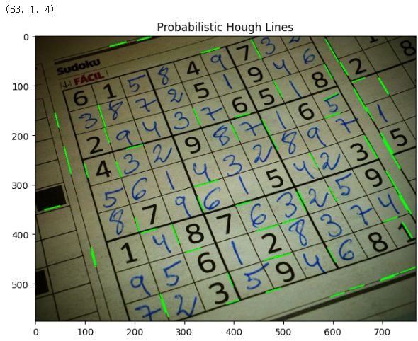
print(lines.shape)의 결과값이 (63, 1, 4)로 출력이 됐는데 이는 NumPy 배열의 형태(Shape)이다.
첫번째 차원(63) : 배열 내 요소의 총 개수
두 번째 차원(1): 각 요소에 대한 하위 배열의 개수
세 번째 차원(4): 하위 배열의 요소 개수
각 선에 대해 네 개의 값(시작점(x1, y1)과 끝점(x2, y2))이 있음을 나타냄
즉, (63, 1, 4) 형태의 배열은 63개의 선을 나타내며, 각 선은 시작점과 끝점의 좌표(x1, y1, x2, y2)를 포함하는 하위 배열을 가지고 있다는 뜻이다.
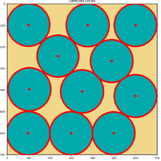
3. Hough Circles
!wget https://raw.githubusercontent.com/rajeevratan84/ModernComputerVision/main/Circles_Packed_In_Square_11.jpeg
image = cv2.imread('Circles_Packed_In_Square_11.jpeg')
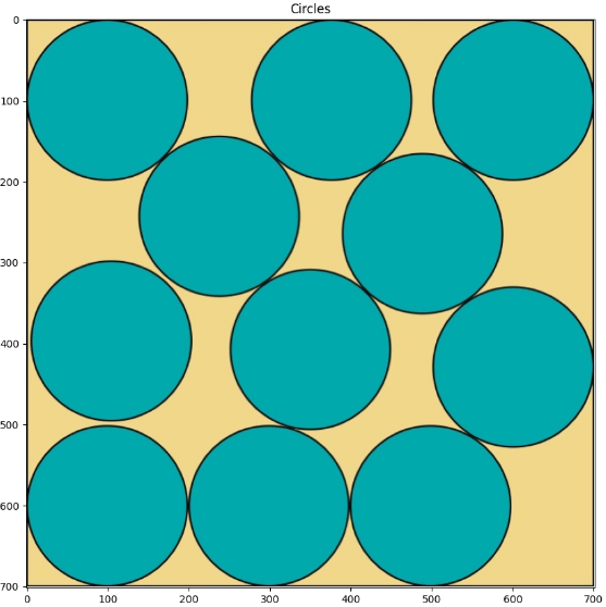
imshow('Circles', image)
gray = cv2.cvtColor(image, cv2.COLOR_BGR2GRAY)
blur = cv2.medianBlur(gray, 5)
circles = cv2.HoughCircles(blur, cv2.HOUGH_GRADIENT, 1.2, 25)
cv2.HoughCircles(gray, cv2.HOUGH_GRADIENT, 1.2, 100)
circles = np.uint16(np.around(circles))
for i in circles[0,:]:
# draw the outer circle
cv2.circle(image,(i[0], i[1]), i[2], (0, 0, 255), 5)
# draw the center of the circle
cv2.circle(image, (i[0], i[1]), 2, (0, 0, 255), 8)
imshow('Detected circles', image)cv2.HoughCircles(image, method, dp, MinDist, param1, param2, minRadius, MaxRadius)이미지에서 원을 검출하는 함수로 사용되며
cv2.HoughCircles(gray, cv2.HOUGH_GRADIENT, 1.2, 100)두번째 인자인 method는 현재 cv2.Hough_gradient 메서드만 지원하므로 해당 코드를 넣어주고
dp는 입력 이미지 해상도에 대한 역비율이다. 값이 클수록 원이 클 수 있다.
마지막 Mindist는 원 중심간의 최소거리이며, 이 값이 작을수록 원 간의 거리가 가깝게 설정된다.
4. Blob Detection(블롭 탐지)
# Read image
image = cv2.imread("images/Sunflowers.jpg")
imshow("Original", image)

# Set up the detector with default parameters.
detector = cv2.SimpleBlobDetector_create()

# Detect blobs.
keypoints = detector.detect(image)

# Draw detected blobs as red circles.
# cv2.DRAW_MATCHES_FLAGS_DRAW_RICH_KEYPOINTS ensures the size of
# the circle corresponds to the size of blob
blank = np.zeros((1,1))
blobs = cv2.drawKeypoints(image, keypoints, blank, (0,255,0),
                                      cv2.DRAW_MATCHES_FLAGS_DEFAULT)

# Show keypoints
imshow("Blobs", blobs)
결과를 보면 해바라기 중간의 점을 블롭(덩어리)을 인식하여 라인을 그린것이 확인된다.
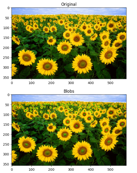
이에 관해선 다음 글에 추가로 작성하겠다.

감사합니다. https://www.youtube.com/channel/UCxlkiu9_aWijoD7BannNM7w