본 글은 2017년 발표된 Neural Collaborative Filtering을 읽고 요약 및 정리한 글입니다.
단어 공부
Auxiliary: 추가적인, 보조적인(간접적인 개념)
- DATA: textual description, acoustic features of music, pictures
- AI: natual language processing, speech recognition, computer vision
0. 핵심요약
- 딥러닝을 추천 시스템에 성공적으로 도입
- [MF] 전통적 행렬분해의 한계
- 내적(Inner Product)의 한계
- user-item interaction을 단순 내적으로만 모델링
- 선형적 패턴만 포착
- 내적(Inner Product)의 한계
- [NeuMF] 딥러닝 모델을 효과적 도입
- GMF: user-item의 저차원 interaction을 모델링
- MLP: 다층 딥러닝을 통해 고차원 interaction을 모델링
- NeuMF: GMF와 MLP를 Joint Training
1. Introduction
- 정보의 홍수 시대에서 추천 시스템은 굉장히 중요
- 특히 MF로 대표되는 Collaborative filtering
- Netflix Prize를 시작으로 MF는 여러가지 방법으로 발전
- Inner product를 이용해서 user-item interaction을 모델링
- complex structure를 모두 잡기엔 충분하지 않음
- Deep Neural Network를 이용해서 이를 해결하고자 함
- 다른 연구에서는 DNN을 이용해서 auxiliary information을 모델링하고자 함
- 여전히 CF 기반 모델은 Inner product에 의존
- 해당 연구에서는 DNN을 Collaborative Ciltering 문제 해결에 사용
2. Preliminaries
2.1. Learning from Implicit Data
- : Observed data(interaction)
- user가 item을 실제로 좋아하는 지 알 수 없음
- noisy signal
- : Unonserved data
- 추천은 unobserved entries를 추론하는 문제
- missing value
- Machine Learning
- Pointwise learning:
- Pairwise learning:
2.2. Matrix Factorization
- MF는 latent vector의 inner product(Linear model)
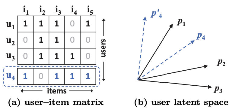
MF(Inner Product)의 한계
(a)를 통해 는 , $ 순으로 유사
하지만 latent space(b)에서 를 과 가장 가깝게 놓으면
가 보다 에 더 가까워지고 더 큰 ranking loss 발생
3. Neural Collaborative Filtering
3.1. General Framework
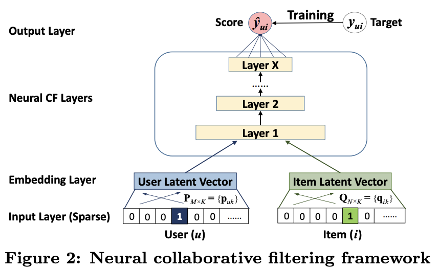
- Predictive model
- NCF with MLP
3.1.1 Learning NCF
- Binary Cross Entropy
implicit feedback의 특성상 은 u와 i가 연관이 있다(반대는 0)
3.2 Generalized Matrix Factorization(GMF)
- MF의 일반화된 형태
여기서 을 identity function 를 uniform function을 사용하면 MF와 정확히 동일
반대로 를 non-linear function 사용하면 더 일반화
3.3 Multi-Layer Perceptron(MLP)
- NCF는 user, item에 대한 2-pathway 모델
- 이는 Multimodal deep learning work에서 흔히 사용
- CF에서 vector concatenation은 interaction을 모델링하기 불충분
- 이를 해결하기 위해 MLP를 도입
- MLP Design
- Activation: ReLU
- Tower Pattern: From wide bottom to smaller nueron
3.4 Fusion of GMF and MLP
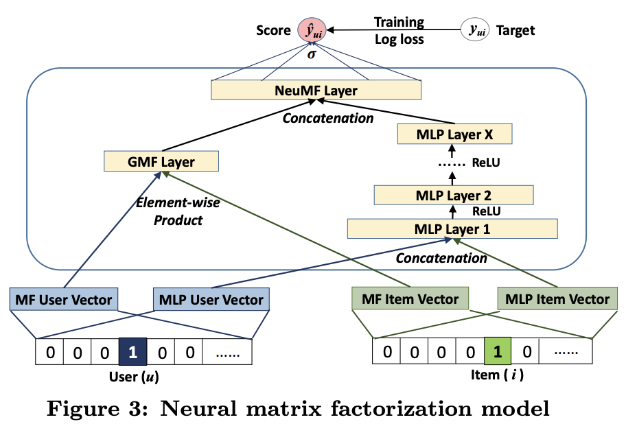
- Embedding Layer 공유
- NTN(Neural Tensor Network)에서 사용
- Performance에 한계가 존재(GMF와 MLP의 embedding size가 동일해야 함)
- Embedding Layer 분리
- NeuMF
- MF(Linear), DNN(Non-linear)
- Adam을 이용했을 때 효과적 학습
4. EXPERIMENT
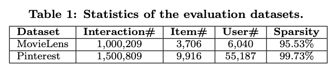
- Dataset
- MovieLens: 최소 20번의 interaction, implicit feedback으로 변환
- MovieLens-1m 다운로드
- Pinterest: 최소 20번의 interaction이 존재하는 데이터만 사용
- Pinterest 다운로드
- Evaluation
- leave-one-out(latest)
- Random 100개의 item을 뽑아 평가
- HR(Hit Ratio)
- NDCG(Normalized Discounted Cumulative Gain)
- top 10
- ItemPop, ItemKNN, BPR, eALS와 비교
- Hyperparameter
- Negative Sampling - 1(Positive) : 4(Negative)
- Model Parameter - Random Initialize
- Adam
- batch size - [128, 256, 512, 1024]
- learning rate - [0.0001, 0.0005, 0.001, 0.005]
- Predictive Factor(last hidden layer) - [8, 16, 32, 64]
- 3 hidden layers
- Predictive Factor: 8 = [32 16 8]
- RQ1. NCF는 SOTA 모델의 성능을 능가할까?
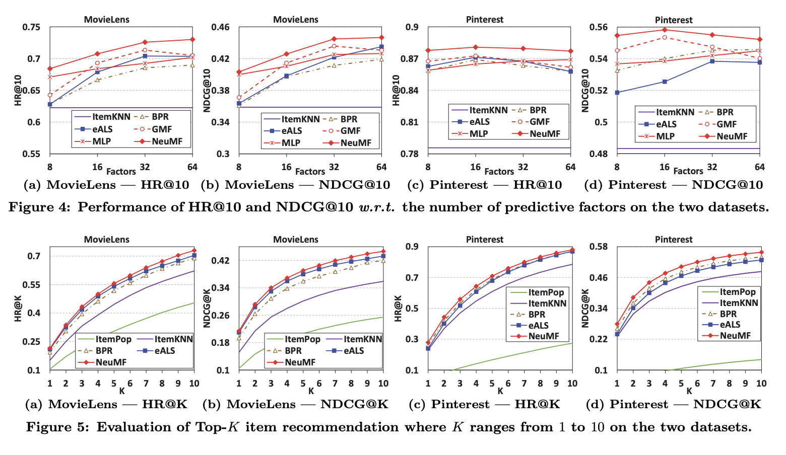
NeuMF가 성능을 모두 이김
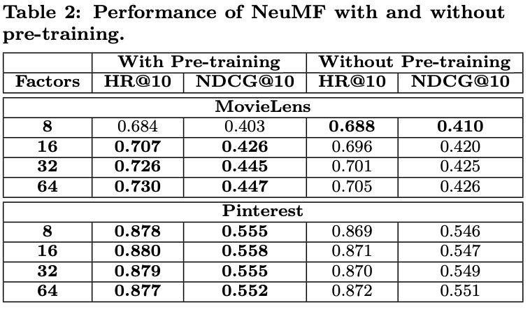
pre-training을 했을 때, 더 좋은 성능을 보임
- RQ2. Negative Sampling을 이용한 logloss 학습
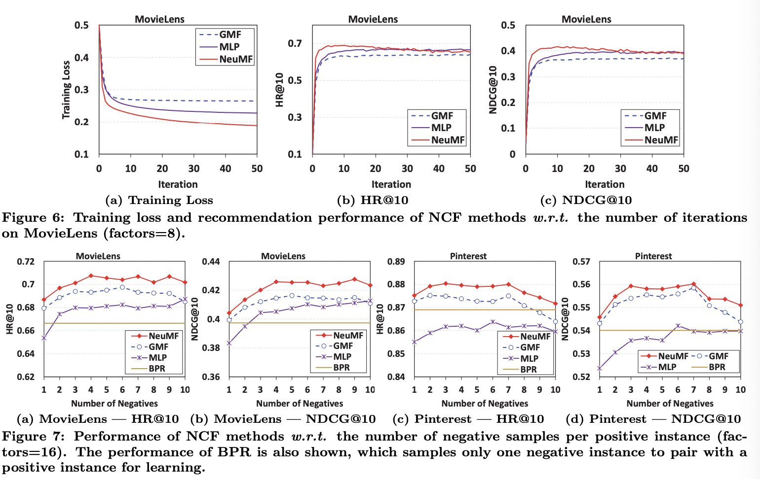
a. 더 많은 interactions가 있을 수록 학습이 잘 됨
b. NeuMF > MLP > GMF
c. 충분한 negative sampling이 필요( > 1)
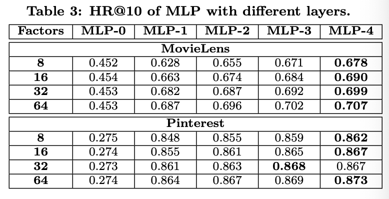
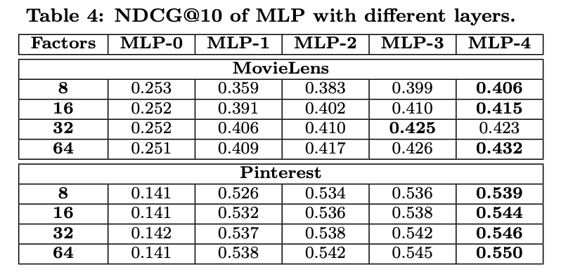
- RQ3. hidden units을 더 깊이 쌓을수록 좋을까?