
💡 Perceptron
The basic unit of a neural network, consisting of a single neuron
🎨 Structure of Perceptron
-
Input Layer
- The input of the perceptron is given in the form of a vector, which can be expressed as
- Each input value is interpreted as a feature, representing the data to be learned
- ex) In the case of image data, can represent the values of each pixel
-
Weights
- Weights are assigned to each input value
- Weights represent the relationship between input and output and are optimized through learning algorithms
-
Bias
- A constant added to the sum of the weighted inputs
-
Weighted Sum
- The linear combination of inputs and weights is calculated as follows:
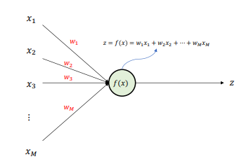
- The linear combination of inputs and weights is calculated as follows:
-
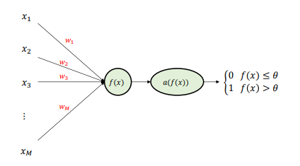
Activation Function
- The perceptron transmits the linearly combined value to the activation function to compute the final output
- The most basic activation function in a perceptron is the step function
- step function: Outputs 1 if is greater than 0, otherwise 0
-
Learning Algorithm
- The perceptron learns through supervised learning
- It updates weights and biases based on the given inputs and their corresponding actual output values (labels)
- Typically, gradient descent is used
🎨 Learning Process of Perceptron
-
Preparing Input Data
- is input, labeled supervised learning data for each input
- The actual label for each input data is denoted as
-
Initializing Weights and Bias
- The perceptron starts by initializing random weights and bias
-
Feedforward
- The linear combination is calculated using the input , current weights , and bias
- The linear combination is calculated using the input , current weights , and bias
-
Error Calculation
- Calculate the error by finding the difference between the actual output and the predicted value
- Calculate the error by finding the difference between the actual output and the predicted value
-
Weight Update
-
Weights and bias are adjusted using the following rule to reduce prediction error:
-
Here, represents the change in weight, which is defined as follows:
- Learning Rate : A hyperparameter that determines how fast the weights are updated; if it's too large, the model becomes unstable, and if it's too small, learning is very slow
- : Error, the difference between the actual and predicted values
- : Input value, the larger the input, the greater the impact on the corresponding weight
-
The bias is updated as follows:
- This formula shows that the bias is updated based on the error, just like the weights
-
-
Iteration
- epoch : The process of calculating output for all inputs in the dataset and updating the weights and bias
- Weight update process:
🎨 Logic Gate
- AND gate : A logic operation where the output is 1 only when both inputs are 1
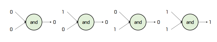
def AND_gate(x1, x2): w1, w2, b = 1, 1, -1.5 # Weight and Bias z = w1 * x1 + w2 * x2 + b return 1 if z > 0 else 0 - NOT gate : Return an inverted output for a single input value
def NOT_gate(x): w, b = -1, 0.5 # Weight and Bias z = w * x + b return 1 if z > 0 else 0 - OR gate : A logic operation where the output is 1 if either input is 1
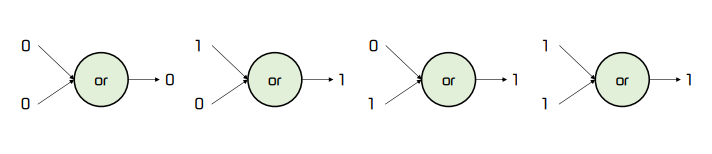
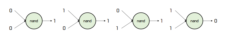
def OR_gate(x1, x2): w1, w2, b = 1, 1, -0.5 # Weight and Bias z = w1 * x1 + w2 * x2 + b return 1 if z > 0 else 0 - XOR gate : Outputs 1 only when the input values are different
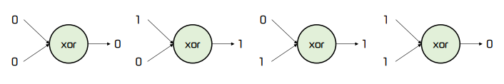
# The XOR gate cannot be implemented with a single perceptron, but can be implemented using a multilayer perceptron def XOR_gate(x1, x2): # Combine AND, OR, and NOT gates to implement the XOR gate s1 = OR_gate(x1, x2) # First Hidden Layer s2 = AND_gate(x1, x2) # Second Hidden Layer y = AND_gate(NOT_gate(s2), s1) # Output Layer return y - The XOR problem cannot be solved with a single perceptron because it is not linearly separable
🎨 Multilayer Perceptron
- Limitations of Perceptron
- Inability to solve nonlinear problems: Perceptrons cannot solve nonlinearly separable problems like the XOR problem
- Difficulty in learning complex patterns: A single perceptron does not have sufficient learning capacity to handle complex problems like image or speech recognition
- Activation function limitation: The basic perceptron uses the step function to determine output, but since this function is not differentiable, it restricts weight optimization
- Structure of Multilayer Perceptron
- Input Layer: The layer that receives data,
- Hidden Layer: Neurons in the hidden layer use nonlinear activation functions to transform data
- Output Layer: Receives the output from the hidden layer to produce the final result
- Operation of Multilayer Perceptron
- Feedforward: Input data starts at the input layer and is propagated sequentially through the hidden layer to the output layer
- Output Generation: The predicted value generated in the output layer is compared to the actual value to calculate the Loss function
- Backpropagation: The process of adjusting weights and biases based on the value of the Loss function
- Backpropagation adjusts weights by propagating errors backward to the input layer
- Weights are updated using optimization algorithms such as Gradient Descent, and the gradient is calculated using the derivative of the loss function
- Gradient Descent: After calculating the gradient of the loss function for each weight through backpropagation, the weights are updated as follows:

Data Analysis