Activation Function

💡 Activation Function

Transform the output of the neural network non-linearly

---

🎨 Activation Function

• Role of the Activation Function

  • Introducing Non-linearity: The neural network can learn complex patterns in input data through non-linear activation functions
  • Determining Neuron Activation: If the input passes through the activation function and exceeds a certain threshold, the neuron gets activated; otherwise, it remains inactive
  • Enabling Learning via Gradient Descent: Activation functions are usually differentiable, and their derivatives are used in backpropagation to compute the gradient of the loss function

• Considerations when Choosing an Activation Function

  • Problem Type: For binary classification problems, Sigmoid or Tanh functions are used; for multi-class classification, Softmax; for regression problems, ReLU or Leaky ReLU are generally used
  • Gradient Vanishing Problem: To solve the gradient vanishing problem, ReLU-based activation functions are commonly used
    • In the backpropagation process, where the gradient of the loss function calculated in the output layer is propagated back to the previous layers, the gradient of each layer is calculated by multiplying the gradient of the previous layer by the weights and the derivative of the activation function in the current layer
    • For example, if the network has 3 layers, the gradient in the output layer is propagated to the previous layer as follows:
      $\frac{\delta L}{\delta w_1} = \frac{\delta L}{\delta a_3} \cdot \frac{\delta a_3}{\delta z_2} \cdot \frac{\delta z_2}{\delta w_1}$
    • If the derivative values are small, the values being multiplied become smaller, and the gradient approaches 0 as it propagates deeper into the network, resulting in almost no learning in the initial layers
  • Depth of the Neural Network: The deeper the neural network, the more sensitive it becomes to the gradient vanishing problem, so ReLU-based functions are more effective

🎨 Sigmoid Function

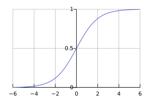
A non-linear function that transforms the input into a value between 0 and 1

• Formula

  $\sigma(x) = \frac{1}{1+e^{-x}}$
  • Here, (x) represents the input, and it can be a real number
  • (e) is the natural constant (approximately 2.718)

• Graph

  

• Derivative of the Sigmoid Function

  $\sigma'(x) = \sigma(x) (1-\sigma(x))$
  • Once the output of the sigmoid function is known, the derivative can be easily calculated

• Characteristics

  • Output Range: The output of the sigmoid function is always between 0 and 1. This allows the output to be interpreted as a probability, which is particularly useful in binary classification problems.
  • Non-linearity: As a non-linear function, the sigmoid introduces non-linearity into the neural network, enabling it to learn complex patterns.
  • S-shaped Curve: The sigmoid function forms an S-shaped curve: if the input is small, the output is close to 0; if the input is large, the output approaches 1.
  • Differentiability: The sigmoid function is differentiable, making it advantageous for learning processes that use the backpropagation algorithm.

• Drawbacks

  • Gradient vanishing problem
  • Slow learning when the output is very close to 0 or 1
  • Non-zero-centered output: The output is always positive, making learning less efficient compared to other activation functions like the Tanh function, which has outputs centered around 0.

🎨 Tanh Function

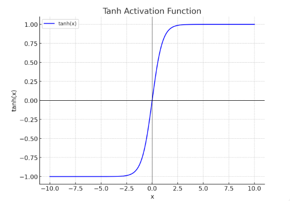
Similar to the Sigmoid function but with an output range between -1 and 1

• Formula

  $tanh(x) = \frac{e^x - e^{-x}}{e^x + e^{-x}}$
  • Here, (e) represents the natural constant (approximately 2.718)

• Graph

  

• Derivative of the Tanh Function

  $\frac{d}{dx} tanh(x) = 1-{tanh}^2 (x)$
  • Once the output of the Tanh function is known, the derivative can also be easily calculated

• Characteristics

  • Output Range: The output range of the Tanh function is between -1 and 1, providing better symmetry than the Sigmoid function
  • Centered around 0: Unlike the Sigmoid function, the Tanh function is centered around 0, meaning that positive inputs return positive outputs, and negative inputs return negative outputs, making it easier for the neural network to learn from data
  • S-shaped Curve: Like the Sigmoid function, the Tanh function forms an S-shaped curve, but it operates over a wider range
  • Non-linearity: As a non-linear function, the Tanh function provides the neural network with the ability to learn complex patterns
  • Differentiability: The Tanh function is differentiable, making it useful in the backpropagation algorithm for gradient calculations during training

• Drawbacks

  • Gradient Vanishing Problem: If the input is very large or very small, the gradient (derivative) of the Tanh function approaches 0, which can lead to the gradient vanishing problem during backpropagation, causing little or no learning
  • Relatively Slower Learning: Although the Tanh function suffers less from the gradient vanishing problem compared to the Sigmoid function, it still has slower learning speed compared to functions like ReLU

🎨 ReLU Function

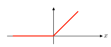
Returns 0 for negative inputs and the input value itself for positive inputs

• Formula

  $f(x) = \max(0, x)$
  • If ( x ) is greater than 0, it outputs ( x ), and if ( x ) is less than or equal to 0, it outputs 0

• Graph

  

• Characteristics

  • Output Range: ReLU returns 0 for negative inputs and outputs the input value itself for positive inputs
  • Non-linearity: Although ReLU is a non-linear function, it is defined much more simply than other non-linear activation functions. However, it still provides non-linearity, allowing the neural network to learn complex patterns when stacking multiple layers
  • Simple Calculation: ReLU involves very few calculations, so it works extremely fast, even in large neural networks
  • Solves Gradient Vanishing Problem: Unlike Sigmoid or Tanh, ReLU maintains a gradient of 1 for positive inputs, helping to mitigate the gradient vanishing problem during backpropagation
  • Induces Sparsity: ReLU sets negative values to 0, leading to the deactivation of some neurons in the network. This effectively simplifies computation by deactivating unnecessary neurons for certain inputs and introduces sparsity in the model

• Drawbacks

  • Dead ReLU Problem:
    • Since ReLU returns 0 for negative inputs, some neurons may end up always outputting 0 during training
    • This can lead to the dead neuron problem, where certain neurons stop contributing to the learning process and become permanently inactive during training

🎨 Leaky ReLU Function

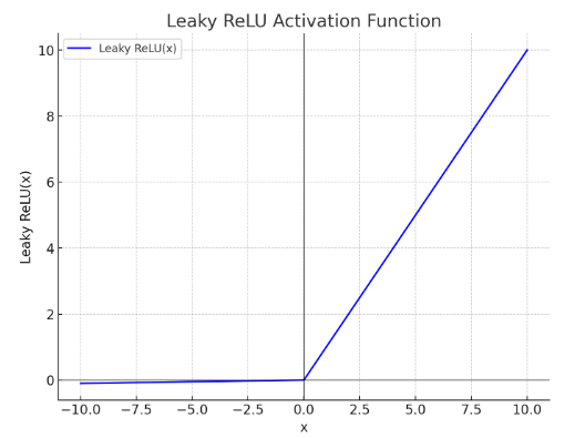
Developed to address the Dead Neurons problem of ReLU, Leaky ReLU applies a small gradient to negative inputs to ensure that all inputs have a non-zero gradient

• Formula

  $f(x) = \begin{cases} x & \text{if } x > 0 \\ \alpha x & \text{if } x \leq 0 \end{cases}$
  • ( \alpha ) is the gradient applied to negative inputs, usually set to a small value like 0.01
  • Since ( \alpha ) is not zero, negative values still contribute to learning with a small gradient

• Graph

  

• Derivative of the Leaky ReLU Function

• Characteristics

  • Output Range: The output of Leaky ReLU is the value ( x ) for positive inputs, and ( \alpha z ) for negative inputs, resulting in an output range of ( (-\infty, \infty) ) with no restrictions
  • Non-linearity, Differentiability
  • Mitigates Dead Neuron Problem: Unlike ReLU, which returns 0 for negative inputs, Leaky ReLU retains a small negative slope for negative inputs, maintaining a small gradient

• Drawbacks

  • Fixed Gradient ( \alpha ): Leaky ReLU uses a fixed gradient ( \alpha ) for negative inputs, and if ( \alpha ) is not appropriately set, it can negatively impact learning, making it important to choose the right ( \alpha ) value
  • More Complex than ReLU: Leaky ReLU is more complex than ReLU and requires setting an additional hyperparameter ( \alpha )

🎨 Softmax Function

Converts input values to values between 0 and 1, and ensures that the sum of these values equals 1 -> Can be interpreted as a probability distribution

• Formula

• Converts the output value ( z_i ) for each class into an exponential function, then divides by the sum of the exponential values of all classes to calculate the probability for each class

  $\sigma(z_i) = \frac{e^{z_i}}{\sum_{j=1}^{K} e^{Z_j}}$
  • ( z_i ) is the input value for class ( i )
  • ( K ) is the total number of possible classes
  • ( e ) is the natural constant

• Characteristics

  • Probability Output: The output value for each class is between 0 and 1, and the sum of the probabilities for all classes equals 1: Softmax converts the input values into a probability distribution
  • Reflects Relative Magnitudes: The larger the input value, the higher the probability for that class; probabilities are calculated based on the relative magnitude of all input values
  • Interdependence Between Classes: When the probability of one class increases, the probabilities of other classes decrease -> Suitable for multi-class classification problems
  • Interpretable Output: The output of the Softmax function can be interpreted as the probability that the data belongs to each class

• How it Works

  1. Convert Logits to Exponential Functions: Convert the logits (output values) of each class to exponential functions

     $e^{z_i}$

  2. Normalization: Divide the exponential value of each class by the total sum of exponential values across all classes, converting the result into probabilities: The sum of probabilities across all classes must equal 1

     $\frac{e^{z_i}}{\sum_{j=1}^{K} e^{Z_j}}$

  3. Probability Calculation: After normalization, the calculated probability for each class represents the likelihood that the data belongs to that class

• Softmax Function Example

  • Suppose there are three classes (A, B, C), and the logits for these classes are ( z_A=2.0 ), ( z_B=1.0 ), and ( z_C=0.1 )

  1. Convert the logits to exponential values

     $e^{z_A} = e^{2.0} \approx 7.39 \\ e^{z_B} = e^{1.0} \approx 2.72 \\ e^{z_C} = e^{0.1} \approx 1.105$

  2. Sum of exponential values for all classes:

     $\sum_{j=1}^{3} e^{z_j} = 7.39 + 2.72 + 1.105 \approx 11.215$

  3. Probability calculation for each class:

     $\sigma(z_A) = \frac{e^{z_A}}{\sum_{j=1}^{3} e^{z_j}} = \frac{7.39}{11.215} \approx 0.659 \\ \sigma(z_B) = \frac{e^{z_B}}{\sum_{j=1}^{3} e^{z_j}} = \frac{2.72}{11.215} \approx 0.242 \\ \sigma(z_C) = \frac{e^{z_C}}{\sum_{j=1}^{3} e^{z_j}} = \frac{1.105}{11.215} \approx 0.099$
  • Therefore, the output of the Softmax function is ( z_A=0.659 ), ( z_B=0.242 ), and ( z_C=0.099 ), representing the probabilities for each class

• Pros and Cons

  • Pros: Probabilistic interpretation, suitable for multi-class classification, well-suited for use in neural networks
  • Interdependence Between Classes:
    • The Softmax function converts the output values of all classes into a single probability distribution
    • If the probability of one class increases, the probabilities of other classes decrease -> This makes it unsuitable if independence between classes is desired
  • Numerical Instability:
    • Exponentiating large values can result in very large numbers, leading to overflow or underflow issues during computation
    • Log-Softmax can be used to address this problem