💡 Regression

A technique for modeling the relationship between multiple independent variables (X) and a single dependent variable (y)

---

🎨 RSS and Gradient Descent

RSS

• A method where the squared error values (Errorᵢ) of each data point are calculated and summed

  $RSS = \sum_{i=1}^{n} (Error_i)^2$

• RSS can be expressed as a function of variables $w_0$ and $w_1$
  , and the key objective of machine learning-based regression is to find the regression coefficients $w_0$ and $w_1$ that minimize this RSS through training

  $RSS(w_0, w_1) = \frac{1}{N} \sum_{i=1}^{N} \left( y_i - \left( w_0 + w_1 \times x_i \right) \right)^2$

• In regression, the Residual Sum of Squares (RSS) is referred to as the cost, and the RSS, composed of the coefficients $w$, is called the Cost Function

• The ultimate goal is to find the minimum value of the cost function, where the error returned by the function no longer decreases. This is also known as the Loss Function.
  
  

Gradient Descent

• Gradient Descent is a method of searching for the 𝑊 parameter that minimizes the error value while updating the 𝑊 parameter value through ‘gradually’ repetitive calculations.
  
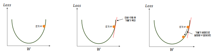
• If the error value no longer decreases, the error value is determined as the minimum cost and the W parameter at that time is returned as the optimal parameter

🎨 Linear Regression

A method for modeling the linear relationship between the independent variable $X$ and the dependent variable $Y$

Simple Linear Regression

• Explain the relationship between a single independent variable $X$ and the dependent variable $Y$

  $Y = \beta_0 + \beta_1 X + \epsilon$

• Here, $\beta_0$ represents the Intercept, $\beta_1$ represents the Slope, and $\epsilon$ represents the Error
  
  

Multiple Linear Regression

• Explains the relationship between multiple independent variables $X_1, X_2, ..., X_p$ and the dependent variable $Y$

  $Y = \beta_0 + \beta_1 X_1 + \beta_2 X_2 + \dots + \beta_p X_p + \epsilon$

• Here, $\beta_0$ represents the Intercept, $\beta_1, \beta_2, ..., \beta_p$ represent the slopes for each independent variable, and $\epsilon$ represents the Error
  
  

Coefficient of Determination ($R^2$)

• One of the key metrics for evaluating the performance of a linear regression model

• Represents the proportion of the variance in the dependent variable that is explained by the independent variables

  $R^2 = 1 - \frac{RSS}{TSS}$

• Here, $RSS$ is Residual Sum of Squares, and $TSS$ is Total Sum of Squares

🎨 Bias-Variance TradeOff

Balancing Bias and Variance for optimal performance

Bias

• A measure of how well the model explains the patterns in the actual data
• A model with high bias fails to capture the complex patterns in the data and provides only a simple approximation -> Underfitting
  
  

Variance

• Indicates how sensitively the model reacts to the training data
• A model with high variance is heavily influenced by small changes in the data, making it overly complex and even learning the noise in the data -> Overfitting

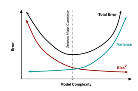
Bias-Variacne TradeOff

• In general, when bias is high, variance tends to be low, and when bias is low, variance is often high
• Looking at the left side of the graph, the model has low complexity, meaning it is not capturing the training data well -> This indicates a state of high bias and low variance, also known as underfitting
• The middle of the graph shows the model finding the optimal balance between bias and variance
• On the right side of the graph, the model is overinterpreting the training data -> Bias is low, but variance is very high, indicating overfitting
  
• Manage this tradeoff through Cross-Validation, Regularization, and Hyperparameter Tuning

🎨 Regularized Linear Regression

A linear regression technique that introduces regularization to prevent overfitting of the model

Lidge Regression

• A linear regression model with L2 regularization -> Adds an extra term to the cost function that minimizes the sum of squared regression coefficients

• Cost Function

  $J(\beta) = \sum_{i=1}^{n} (Y_i - \hat{Y_i})^2 + \lambda \sum_{j=1}^{p} \beta_j^2$

• Here, $\lambda$ is a hyperparameter that controls the strength of regularization. The larger $\lambda$ gets, the greater the penalty, making the model simpler. $\beta_j$ represents the regression coefficients for each independent variable

• Characteristics

  • Brings all regression coefficients closer to 0 but doesn't make them exactly 0
  • Useful for solving multicollinearity problems -> When there is a strong correlation between independent variables, Ridge Regression improves model stability

Lasso Regression

• A linear regression model with L1 regularization -> Adds a penalty based on the sum of the absolute values of the regression coefficients

• Cost Function

  $J(\beta) = \sum_{i=1}^{n} (Y_i - \hat{Y_i})^2 + \lambda \sum_{j=1}^{p} |\beta_j|$

• Here, $\lambda$ is a hyperparameter that controls the strength of regularization, and $|\beta_j|$ represents the absolute value of each regression coefficient

• Characteristics

  • Lasso Regression allows the coefficients to fully shrink to 0 through the $\sum_{j=1}^{p} |\beta_j|$ term
  • Feature Selection: Automatically eliminates unnecessary variables, enabling the creation of a more streamlined model

Elastic Net Regression

• The method that combines Ridge Regression and Lasso Regression

• Cost Function

  $J(\beta) = \sum_{i=1}^{n} (Y_i - \hat{Y_i})^2 + \lambda_1 \sum_{j=1}^{p} |\beta_j| + \lambda_2 \sum_{j=1}^{p} \beta_j^2$

• Here, $\lambda_1$ is the hyperparameter controlling the strength of L1 regularization, and $\lambda_2$ is the hyperparameter controlling the strength of L2 regularization

• Characteristics

  • Useful when the data has high-dimensional features or when multicollinearity is significant
  • Enables feature selection through L1 regularization while ensuring model stability with L2 regularization

The role of regularization strength $\lambda$

• $\lambda$ is a hyperparameter that controls the strength of regularization, with larger values applying stronger regularization
  • $\lambda = 0$: No regularization is applied, making it equivalent to standard linear regression
  • If $\lambda$ is too large, the model can become overly simplified, leading to underfitting
  • Finding the right $\lambda$ value helps optimize the bias-variance tradeoff of the model

🎨 Logistic Regression

A regression technique used to solve Binary Classification problems, typically used when the dependent variable is categorical, and mainly for predicting the probability of a specific event occurring

Logistic Function

• If data is predicted using a simple straight line like in linear regression, the predicted values can exceed 0 and 1, which doesn't align with categorical variables (0 or 1)

• Therefore, logistic regression uses a logistic function that converts predicted values into values between 0 and 1

  $h_{\theta}(x) = \frac{1}{1 + e^{-(\theta^T x)}}$

• Here, $h_0(x)$ represents the output probability for input $x$ (between 0 and 1), and $\theta^Tx$ is the linear combination of independent variables and regression coefficients (the predicted value in linear regression). $e$ is the natural constant (approximately 2.718)

• This function has the characteristic that when $\theta^Tx$ is negative, it approaches 0, and when it is positive, it approaches 1 -> The logistic function converts any real number into a probability between 0 and 1

• In logistic regression, the output value can be interpreted as the probability of an event occurring

• In other words, $h_\theta(x)$ represents the probability that the dependent variable $y=1$, while $1-h_\theta(x)$ represents the probability that $y=0$

  $P(y = 1 \mid x; \theta) = h_{\theta}(x)$

Decision Boundary

• In Logistic Regression, if the predicted probability is greater than 0.5, it classifies as $y=1$, and if it is less than 0.5, it classifies as $y=0$

  $\hat{y} = \begin{cases} 1 & \text{if } h_{\theta}(x) \geq 0.5 \\ 0 & \text{if } h_{\theta}(x) < 0.5 \end{cases}$

• Here, $\hat{y}$ represents the predicted class (0 or 1) and $h_\theta(x)$ is the predicted probability value for the independent variable $x$

Logistic Regression in scikit-learn

• Basic Code

from sklearn.linear_model import LogisticRegression
from sklearn.model_selection import train_test_split
from sklearn.datasets import load_iris

# Load data (Iris dataset)
iris = load_iris()
X = iris.data
y = iris.target

# Split data into training and testing sets
X_train, X_test, y_train, y_test = train_test_split(X, y, test_size=0.3, random_state=42)

# Initialize the model
logreg = LogisticRegression()

# Train the model
logreg.fit(X_train, y_train)

# Make predictions
y_pred = logreg.predict(X_test)

# Evaluate performance (Accuracy)
from sklearn.metrics import accuracy_score
print("Accuracy:", accuracy_score(y_test, y_pred))

• Main Hyperparameters
  • penalty : Regularization method selection
    - Default: L2, Options: L1, L2, elasticnet, none
  • C : Regularization strength (inverse regularization coefficient)
    • Default: 1.0, Larger values mean weaker regularization, and smaller values mean stronger regularization
  • solver : Optimization algorithm selection
    • Default: lbfgs, Options: liblinear, lbfgs, saga, newton-cg

🎨 Tree-based Regression

A regression method that uses Decision Trees to predict continuous values, a nonlinear regression model that predicts values based on input variables by repeatedly splitting the data

Decision Tree Regression

• Data splitting -> Split criterion selection: Each split is made in the direction that minimizes variance, meaning the data within each region is split to be as uniform as possible -> Prediction output: The predicted value is returned as the average or median of the data in the node

• In Decision Tree Regression, the loss function is defined as the Residual Sum of Squares

  $RSS = \sum_{i \in R_m} (y_i - \hat{y}_{R_m})^2$

• Here, $y_i$ is the actual dependent variable value, and $\hat{y}_{R_m}$ is the predicted value (mean) for region $R_m$ -> The model splits the data by minimizing RSS

Random Forest Regression

• An ensemble learning method based on decision trees
• Key concepts
  • Ensemble: Trains multiple decision trees and combines their predictions to generate the final prediction value
  • Bagging: Trains each tree using only a subset of the data through bootstrap sampling
  • Randomness introduction: When training each tree, only a random subset of features is selected as the split criterion -> Reduces correlation between trees, resulting in better performance

Gradient Boosting Regression

• An ensemble learning method based on decision trees
• Key concepts
  • Boosting: Sequentially trains models, where each subsequent model corrects the errors of the previous model
  • Residual Learning: Each tree learns the residuals (errors) not captured by the previous tree, gradually improving the overall model performance

Tree-based Regression의 비교

Model	Overfitting Risk	Training Speed	Prediction Performance	Interpretability	Computational Cost
Decision Tree Regression	High	Fast	Medium	Very High	Low
Random Forest Regression	Low	Medium	High	Low	Medium
Gradient Boosting	Low (requires tuning)	Slow	Very High	Low	High

🎨 Regression Metrics

Used to evaluate the performance of a regression model

MSE (Mean Squared Error)

• The average of the squared differences between the predicted values and the actual values, sensitive to large errors

  $MSE = \frac{1}{n} \sum_{i=1}^{n} (y_i - \hat{y_i})^2$

• Here, $y_i$ is the actual value, $\hat{y}_i$ is the predicted value, and $n$ is the number of data points

• Characteristics

  • The closer the value is to 0, the closer the model's predictions are to the actual values
  • Sensitive to large errors, and the presence of outliers can cause MSE to increase significantly

MAE (Mean Absolute Error)

• The average of the absolute differences between the predicted values and the actual values, less sensitive to outliers since it does not square the differences

  $MAE = \frac{1}{n} \sum_{i=1}^{n} |y_i - \hat{y_i}|$

• Characteristics

  • A metric that allows for an intuitive interpretation of how far predictions are from the actual values
  • Less sensitive to outliers, providing a more stable evaluation when there are large errors in the data
    
    

$R^2$ (Coefficient of Determination)

• Evaluates how well the model's predictions explain the variability in the actual data

  $R^2 = 1 - \frac{ \sum_{i=1}^{n} (y_i - \hat{y_i})^2 }{ \sum_{i=1}^{n} (y_i - \bar{y})^2 }$

• Here, $y_i$ is the actual value, $\hat{y}_i$ is the predicted value, $\bar{y}$ is the mean of the actual values, and $\sum_{i=1}^{n} (y_i - \bar{y})^2$ represents TSS, which indicates the total variability of the data

• Characteristics

  • $R^2 = 1$ -> The model perfectly predicts all the data
  • $R^2 = 0$ -> The model does not explain any of the variability in the data
  • Negative values can occur, indicating that the model performs worse than simply predicting the mean

RMSE (Root Mean Squared Error)

• The square root of MSE, representing the difference between actual and predicted values in the original units

  $RMSE = \sqrt{\frac{1}{n} \sum_{i=1}^{n} (y_i - \hat{y_i})^2}$

• Characteristics

  • Sensitive to large errors
  • Easier to interpret since it is expressed in the original units of the data
  • Generally, a smaller RMSE value indicates that the model's predictions are more accurate

MSLE (Mean Squared Logarithmic Error)

• The mean of the squared errors of the logarithmic differences between the predicted values and the actual values

  $MSLE = \frac{1}{n} \sum_{i=1}^{n} \left( \log(1 + y_i) - \log(1 + \hat{y_i}) \right)^2$

• Characteristics

  • Particularly useful when the range of values is large
  • More sensitive to smaller values, making it helpful when emphasizing prediction accuracy for smaller values over larger ones