💡 Ensemble

To obtain more reliable predictions than a single classifier by combining the prediction results of various classifiers

---

🥨 Voting

Combining classifiers with different algorithms

Hard Voting

• Definition : Final class determination through majority voting among multiple classifiers
• Example : If three models predict classes A, B, and A, respectively, the final prediction would be A (because it received the majority of votes)

Soft Voting

• Definition : Determine by averaging the class probabilities of multiple classifiers; commonly used
• Example : If three models predict the probabilities for class A as 0.6, 0.7, and 0.8, the average probability for class A would be 0.7, and if this is the highest among all classes, A would be the final prediction

Implementation Details

• Homogeneous vs. Heterogeneous Models : Voting can be applied to both homogeneous models (models of the same type, such as multiple decision trees) and heterogeneous models (different types of models, such as a decision tree, a logistic regression model, and an SVM)
• Weights : In soft voting, weights can be assigned to each model to reflect their importance or accuracy. More accurate models may be given higher weights, influencing the final prediction more strongly

🥨 Bagging

• Definition : Combine classifiers with the same algorithm, perform data sampling differently during training, and then conduct voting
• How Bagging works
  1. Bootstrap Sampling
     • Bagging starts by creating multiple subsets of the original training data. Each subset is generated by randomly sampling the data with replacement, meaning some data points may be repeated in a subset, while others may be left out.
  2. Training Multiple Models
     • For each bootstrap sample, a separate model (referred to as a base model or weak learner) is trained. These models are typically of the same type, such as decision trees.
     • Since each model is trained on a different subset of the data, they are likely to learn slightly different patterns, even if they are using the same algorithm.
  3. Aggregation of Predictions
     • After training, the predictions from all the base models are combined to produce the final prediction.

Random Forest

• Definition : Multiple decision tree classifiers individually sample data from the entire dataset using the bagging method, train separately, and then ultimately make predictions through voting by all classifiers; a representative algorithm of bagging

• Main Hyperparameters

  • n_estimators : The number of trees in the forest; Increasing the number of trees generally improves performance but also increases computational cost
  • max_features : The number of features to consider when looking for the best split; auto (which means sqrt(n_features) for classification and n_features for regression)
  • max_depth : The maximum depth of each tree
  • min_samples_leaf : The minimum number of samples required to be at a leaf node
  • min_samples_split : The minimum number of samples required to split an internal node

• Basic Python Code to Implement a Random Forest

  # Import necessary libraries
  from sklearn.datasets import load_iris
  from sklearn.model_selection import train_test_split
  from sklearn.ensemble import RandomForestClassifier
  from sklearn.metrics import accuracy_score
  
  # Load the Iris dataset
  iris = load_iris()
  X = iris.data
  y = iris.target
  
  # Split the dataset into training and testing sets
  X_train, X_test, y_train, y_test = train_test_split(X, y, test_size=0.3, random_state=42)
  
  # Create a Random Forest Classifier
  rf_classifier = RandomForestClassifier(n_estimators=100, random_state=42)
  
  # Train the model
  rf_classifier.fit(X_train, y_train)
  
  # Make predictions on the test set
  y_pred = rf_classifier.predict(X_test)
  
  # Calculate the accuracy of the model
  accuracy = accuracy_score(y_test, y_pred)
  print(f"Accuracy: {accuracy:.2f}")

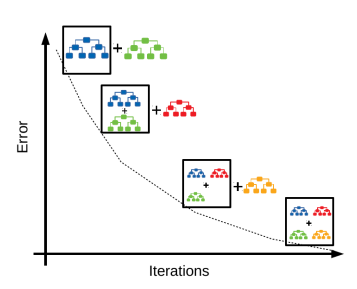
🥨 Boosting

A method in which multiple weak learners are sequentially trained, with the learning process involving assigning weights to the predicted data or decision trees to correct errors as learning progresses

AdaBoost(Adaptive Boosting)

• Definition : An ensemble learning technique that combines multiple weak learners to form a strong classifier. It is primarily used for classification tasks and works by sequentially training models while focusing on the errors made by previous models.

• How AdaBoost Works

  1. Initialize Weights : All training instances start with equal weights
  2. Train Weak Leaners : A sequence of weak learners (e.g., decision stumps) is trained. After each learner is trained, the instances it misclassified are given higher weights.
  3. Update Weights : Misclassified instances have their weights increased, ensuring that the next learner focuses more on these instances
  4. Combine Learners : Each learner’s prediction is weighted according to its accuracy. The final model is a weighted combination of all the learners
  5. Iterate : The process is repeated for a specified number of iterations or until the error is minimized

• Chracteristics

  • Sequential Learning : Unlike methods like bagging, AdaBoost trains models sequentially, with each new model attempting to correct the errors of the previous ones
  • Focus on Hard Cases : AdaBoost increases the weights of misclassified instances so that subsequent learners focus more on these difficult cases
  • Semsitivity to Noise : AdaBoost can be sensitive to noisy data or outliers because it increases the weight of misclassified instances
  • No Parameter Tuning : Generally requires fewer parameters to tune compared to other ensemble methods

• AdaBoost in Python

  from sklearn.ensemble import AdaBoostClassifier
   from sklearn.datasets import load_iris
   from sklearn.model_selection import train_test_split
   from sklearn.metrics import accuracy_score
  
   # Load the Iris dataset
   iris = load_iris()
   X = iris.data
   y = iris.target
  
   # Split the dataset into training and testing sets
   X_train, X_test, y_train, y_test = train_test_split(X, y, test_size=0.3, random_state=42)
  
   # Create an AdaBoost classifier
   ada_classifier = AdaBoostClassifier(n_estimators=50, random_state=42)
  
   # Train the model
   ada_classifier.fit(X_train, y_train)
  
   # Make predictions on the test set
   y_pred = ada_classifier.predict(X_test)
  
   # Calculate accuracy
   accuracy = accuracy_score(y_test, y_pred)
   print(f"Accuracy: {accuracy:.2f}")

GBM (Gradient Boost Machine)

• Definition : Similar to AdaBoost, but the weight updates are performed using gradient descent
  
• Gradient Descent
  • A technique that derives the update values for weights to minimize errors through iterative execution
  • Where the feature $x$ is input, the model's prediction fuctions is $F(x)$ and the actual target value is $y$, then the error function $h(x) = y-F(x)$. In this case, the weights are iteratively updated in the direction that minimizes $h(x)$.
• Main Hyperparameters
  • loss : Specify the Loss Function
  • learning_rate : The coefficient applied by the weak learner to sequentially correct the error values, typically specified as a value between 0 and 1
  • n_estimators : The number of weak learners
  • subsample : The sampling rate of the data used by the weak learner for training, default is 1.

XGBoost (eXtra Gradient Boost)

• Characteristics
  • Designed for high performance; Optimized for speed and memory usage, making it suitable for large datasets
  • Faster execution time compared to GBM, supports CPU parallel processing, and GPU acceleration
  • RProvides regularization and tree pruning features
  • Supports early stopping, built-in cross-validation, and handles missing values natively
• Early Stopping in XGBoost
  • If the loss function does not decrease for a specified number of iterations, the execution stops without completing the total number of iterations
  • Be cautious, as shortening the number of iterations too much may cause the training to stop before the model's predictive performance is fully optimized
  • Early Stopping setting Parameter
    • early_stopping_rounds : The maximum number of iterations during which the loss evaluation metric does not decrease
    • eval_metric : The cost evaluation metric used during iterative execution
    • eval_set : Set a separate validation dataset for evaluation; typically, the loss reduction performance is evaluated iteratively on the validation dataset

LightGBM

• Characteristics
  • Advantages compared to XGBoost
  • Faster training and prediction execution times
  • Lower memory usage
  • Automatic conversion and optimal splitting of categorical features (converts categorical features optimally without using One-Hot Encoding and performs corresponding split nodes)
• How LightGBM works
  
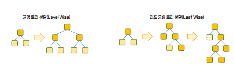
  • Level Wise : The traditional GBM approach, including XGBoost, creates balanced trees to minimize depth. This implementation is based on the theoretical premise that if the tree extends too far in one direction, it could lead to overfitting.
  • Leaf Wise : If predicting in one direction reduces the prediction error, the algorithm determines that continuing to generate leaf nodes in that direction would result in a more accurate model.

🥨 Stacking

• Definition : Unlike simpler ensemble methods like bagging or boosting, involve training a meta-model to learn how to best combine the predictions of several base models
• How Stacking Works
  1. Base Models (Level 0 Models)
     • Multiple different models (such as decision trees, logistic regression, support vector machines, etc.) are trained on the same dataset. These are often referred to as "level 0" models
     • The goal is to leverage the strengths of different algorithms, each capturing various aspects of the data
  2. Meta-Model (Level 1 Model)
     • Once the base models are trained, their predictions (often the predicted probabilities) are used as input features to train a new model, known as the meta-model or level 1 model
     • The meta-model learns the best way to combine these predictions to produce a final output
  3. Training Process
     • Typically, the dataset is split into several parts. The base models are trained on one part of the data, and their predictions are made on the unseen part. These predictions are then used to train the meta-model.
     • This process helps the meta-model generalize well, as it learns from the out-of-sample predictions of the base models.
  4. Prediction
     • During prediction, the base models are applied to the test data to generate predictions. These predictions are then fed into the meta-model, which produces the final prediction.

🥨 Pros and Cons of Ensemble Methods

Advantages of Ensemble Methods

• Improved Accuracy : By combining multiple models, ensembles can achieve higher accuracy than individual models
• Reduced Overfitting : Ensembles can help mitigate overfitting by averaging out the errors of individual models
• Robustness : They provide more stable predictions, as the impact of any single model's errors is minimized

Disadvantages of Ensemble Methods

• Increased Complexity : Ensemble methods are generally more complex and computationally intensive than individual models
• Interpretability : They can be harder to interpret compared to simpler models like a single decision tree