Scientific Python 1

송하·2023년 5월 29일

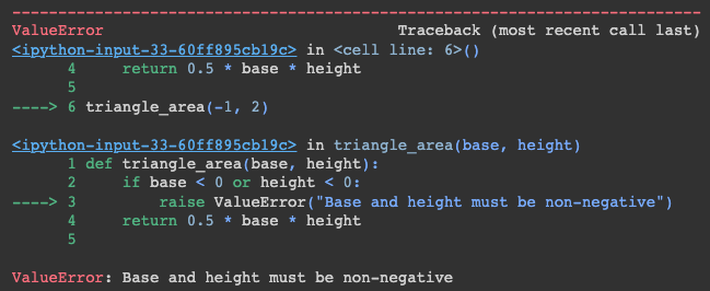
- Pyhton Exceptions

def triangle_area(base, height):
    if base < 0 or height < 0:
        raise ValueError("Base and height must be non-negative")
    return 0.5 * base * height

triangle_area(-1, 2)

이 코드를 돌리면 아래와 같이 에러를 출력해준다.

- Python Object

# everything in python is an object, and can be passed into a function
def f(x):
    return x+2

def twice(f, x):
    return f(f(x))

twice(f, 2) # + 4

파이썬에서는 아무거나 전부 객체로 받을 수 있고 함수로 넘겨준다. → 함수도 객체로 넘겨줄 수 있다.

- List Comprehensions

# 1
S = []
for i in range(2):
    for j in range(2):
        for k in range(2):
            S += [(i,j,k)]

# 2
S = [(i,j,k) for i in range(2) for j in range(2) for k in range(2)]

1번과 2번 코드는 같은 코드다. 파이썬의 목록 이해를 통해 집합 표기법을 연상시키는 방식으로 목록을 만들 수 있다.

- NumPy

x @ y  # Matrix multiplication
# array([[ 0,  4],
#        [ 4, 20]])

@는 Matrix mutiplication을 하기 위한 기호이다.

- Function execution time

%%timeit
x = np.random.rand(10000)
y = np.random.rand(10000)
z=0
for i in range(10000):
    z += x[i]*y[i]

%%timeit은 시간을 재주는 함수이다. 아래 사진과 같이 출력된다. %는 line command로 하나의 라인에 대해서 적용되고 %%는 cell command로 해당 cell에 작성된 모든 코드에 적용된다.
→ 주피터노트북에서 하나의 셀에 대해 수행되는 속도를 측정할 수 있다.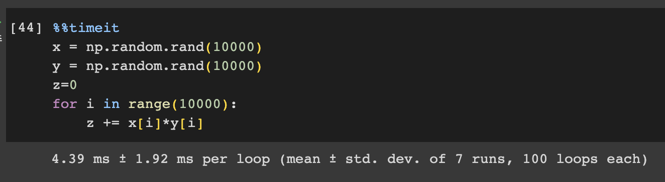

- Generating random numbers

np.random.randint(): 균일 분포의 정수 난수 1개 생성
np.random.rand(): 0부터 1사이의 균일 분포에서 난수 matrix array 생성
np.random.randn(): 가우시안 표준 정규 분포에서 난수 matrix array 생성
np.linspace(): 인자 3개를 기본으로 가진다.
→ (구간 시작점, 구간 끝점, 구간 내 숫자 개수)
```
import numpy as np
 np.linspace(0,5,10)
```

- Initializing functions

#1
5*np.ones((10,10))

#2
np.ones((10,10))*5

#3
np.zeros((10,10)) + 5

1번과 2번 코드는 같은 코드이다. 3번처럼 np.zeros로 0으로 초기화하고 5만큼 더해주면 1,2,3번의 출력값이 서로 같음을 알 수 있다.

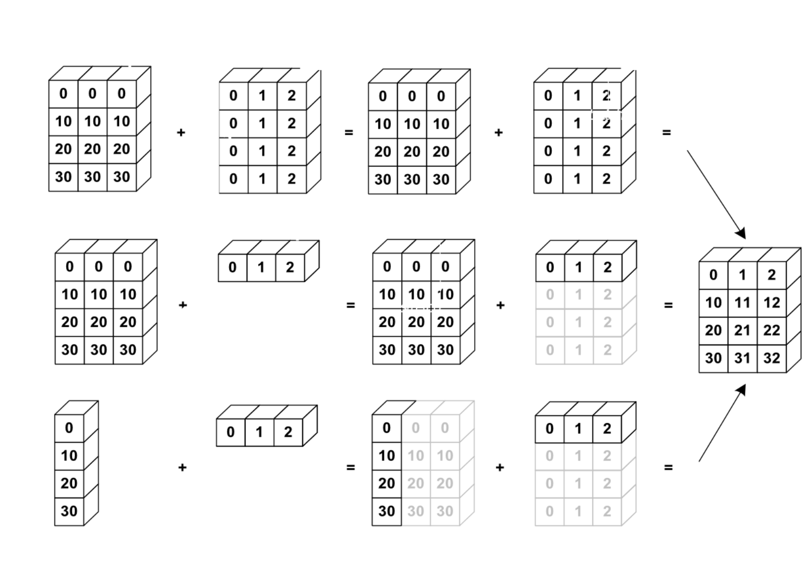
- Numpy Broadcasting

#1
np.arange(10).reshape(10,1)
'''출력값
array([[0],
       [1],
       [2],
       [3],
       [4],
       [5],
       [6],
       [7],
       [8],
       [9]])
'''       

#2
np.arange(10).reshape(10,1)*np.ones((10,10))
'''출력값
array([[0., 0., 0., 0., 0., 0., 0., 0., 0., 0.],
       [1., 1., 1., 1., 1., 1., 1., 1., 1., 1.],
       [2., 2., 2., 2., 2., 2., 2., 2., 2., 2.],
       [3., 3., 3., 3., 3., 3., 3., 3., 3., 3.],
       [4., 4., 4., 4., 4., 4., 4., 4., 4., 4.],
       [5., 5., 5., 5., 5., 5., 5., 5., 5., 5.],
       [6., 6., 6., 6., 6., 6., 6., 6., 6., 6.],
       [7., 7., 7., 7., 7., 7., 7., 7., 7., 7.],
       [8., 8., 8., 8., 8., 8., 8., 8., 8., 8.],
       [9., 9., 9., 9., 9., 9., 9., 9., 9., 9.]])
'''

브로드캐스팅은 어떤 조건만 만족한다면 모양이 다른 배열끼리의 연산도 가능하게 해주며 모양이 부족한 부분은 확장하여 연산을 수행할 수 있도록 한다는 것이라고 생각할 수 있다. 확장 또는 전파한다는 의미로 Broadcasting을 설명하는 가장 간단한 예는 배열과 스칼라 값을 계산하는 것이다.

- np.squeeze()

Z=np.arange(10).reshape(1,-1)
print(Z)
print(Z.shape)
'''출력값
[[0 1 2 3 4 5 6 7 8 9]]
(1, 10)
'''

Z.squeeze()
'''출력값: array([0, 1, 2, 3, 4, 5, 6, 7, 8, 9])'''

squeeze() 함수는 넘파이 배열에서 크기가 1인 추가 axis를 제거하는 함수이다.

- np.eye(), np.diag(), Array.T

np.eye(10) #identity 행렬과 유사
# 차이는 Identity 행렬은 항상 nxn의 행렬이라면, eye는 원하는 NxM으로 행렬을 만들 수 있다.
'''출력값
array([[1., 0., 0., 0., 0., 0., 0., 0., 0., 0.],
       [0., 1., 0., 0., 0., 0., 0., 0., 0., 0.],
       [0., 0., 1., 0., 0., 0., 0., 0., 0., 0.],
       [0., 0., 0., 1., 0., 0., 0., 0., 0., 0.],
       [0., 0., 0., 0., 1., 0., 0., 0., 0., 0.],
       [0., 0., 0., 0., 0., 1., 0., 0., 0., 0.],
       [0., 0., 0., 0., 0., 0., 1., 0., 0., 0.],
       [0., 0., 0., 0., 0., 0., 0., 1., 0., 0.],
       [0., 0., 0., 0., 0., 0., 0., 0., 1., 0.],
       [0., 0., 0., 0., 0., 0., 0., 0., 0., 1.]])
'''

M = np.diag(np.arange(10))
# diag 함수는 parameter로 전달받은 행렬의 k번째 열부터 있는 대각선의 값들을 1차원 array로 반환하는 함수
'''출력값
array([[0, 0, 0, 0, 0, 0, 0, 0, 0, 0],
       [0, 1, 0, 0, 0, 0, 0, 0, 0, 0],
       [0, 0, 2, 0, 0, 0, 0, 0, 0, 0],
       [0, 0, 0, 3, 0, 0, 0, 0, 0, 0],
       [0, 0, 0, 0, 4, 0, 0, 0, 0, 0],
       [0, 0, 0, 0, 0, 5, 0, 0, 0, 0],
       [0, 0, 0, 0, 0, 0, 6, 0, 0, 0],
       [0, 0, 0, 0, 0, 0, 0, 7, 0, 0],
       [0, 0, 0, 0, 0, 0, 0, 0, 8, 0],
       [0, 0, 0, 0, 0, 0, 0, 0, 0, 9]])
'''

A = np.arange(15).reshape(5,3)
'''출력값
array([[ 0,  1,  2],
       [ 3,  4,  5],
       [ 6,  7,  8],
       [ 9, 10, 11],
       [12, 13, 14]])
'''
A = np.arange(15).reshape(5,3).T
# 전치 행렬 구하기 위한 함수
'''출력값
array([[ 0,  3,  6,  9, 12],
       [ 1,  4,  7, 10, 13],
       [ 2,  5,  8, 11, 14]])
'''

- Fancy Array Indexing

idx = np.array([7,-5,2])
arr[idx]=-1
arr
# 출력: array([ 0,  1, -1,  3,  4, -1,  6, -1,  8,  9])

arr[arr<0] = np.arange(3)
arr
# 출력: array([0, 1, 0, 3, 4, 1, 6, 2, 8, 9])