머신러닝 - Multivariate Linear Regression

Multivariate Linear Regression

실제 상황에서는 하나의 변수만으로 예측하기 어려움

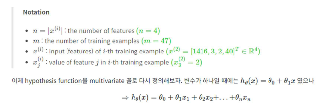
집값 추정 문제의 hypothesis를 ${h_\theta}$(x) = ${80 + 0.1x_1+0.01x_2+3x_3+2x_4}$ 와 같이 나타내고:

• ${\theta_0}$ = 80은 기본 집값
• ${\theta_1}$ = 0.1은 제곱미터당 가격
• ${\theta_2}$ = 0.01은 층당 가격
  ...

로 볼 수 있다.

Matrix multiplication을 통한 hypothesis function

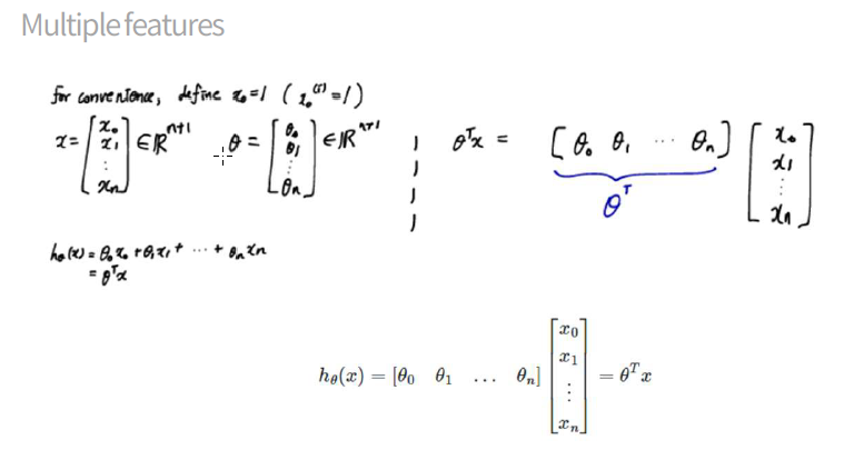
1) 계산을 편하게 하기 위해 $x_0$ = 1

• ${\theta_0 + \theta_0x_1 + \theta_2x_2}$ 를
  ${\theta_0x_0 + \theta_0x_1 + \theta_2x_2}$같은 형태로 만들기 위해서

2) x를 벡터로 표현(입력데이터=feature를 벡터로)하고 ${\theta}$(파라미터, 모델의 weight들)도 벡터로 표현

3) 이 두 벡터를 서로 곱한다.
곱하기 위해 transpose (세로 벡터를 가로로)

4) 곱한 결과: ${h_\theta}(x) = {\theta^Tx}$

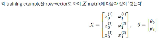
위와 같이 행렬을 이용해 표시하면:
${h_\theta}(x) = X{\theta}$

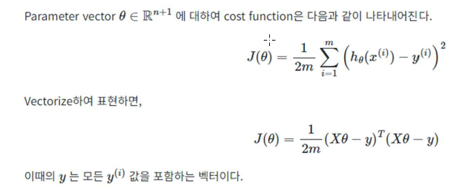
Cost Function:

예제

PyTorch 에서 model은ㅇ Module 클래스로부터 상속된 클래스로 만든다.

가장 기본적으로 두 개 method를 구현해야한다.

• __init__(self)
• forward(self, x)

forward(x) 메서드를 직접 호출하지 않는다. model(x)와 같이 전체 model을 호출한다.

class ManualLinearRegressor(nn.Module):
	def __init__(self):
    super().__init__()
    
    self.a = nn.Parameter(torch.rand(1, requires_grad=True, dtype=torch.float)
    self.b = nn.Parameter(torch.rand(1, requires_trad=True, dtype=torch.gloat))
    
    def forward(self, x):
    	return self.a + self.b*x
        
model = ManualLinearRegressor().to(device)

print(model.state_dict())

loss_fn = nn.MSELoss(reduction='mean')
optimizer = optim.SGD(model.parameters(), lr=lr)

for epoch in range(n_epochs):
	model.train()
    
    yhat = model(x_train_tensor)
    
    loss = loss_fn(yhat, y_train_tensor)
    loss.backward()
    optimizer.step()
    optimizer.zero_grad()

수동으로 linear regression parameter를 생성하는 대신 PyTorch의 Linear 모델을 만들어 nested model 생성

class LasyerLinearRegressor(nn.Module):
	def __init__(self):
      super().__init__()
      self.linear = nn.Linear(in_feaures=1, out_features=1)
    
    def forward(self, x):
    	return self.linear(x)

Sequential model을 이용하면 class 생성도 불필요

model=nn.Sequential(nn.Linear(in_features=1, out_features=1)).to(device)

loop 일반화

def make_train_step(model, loss_fn, optimizer):

	def train_step(x,y):
    	#Sets model to train mode
        model.train()
        
        #Make predictions
        yhat = model(x)
        
        # Compute loss
        loss = loss_fn(yhat, y)
        
        # Compute gradients
        loss.backward()
        
        # Update parameters and zero gradients
        optimizer.step()
        optimizer.zero_grad()
        
        # Return the loss
        return loss.item()
    
   return train_step

model=nn.Sequential(nn.Linear(in_features=1, out_features=1)).to(device)
loss_fn = nn.MSELoss(reduction='mean')
optimizer = optim,SGD(model.parameters(), lr=lr)

train_step=make_train_step(model, loss_fn, optimizer)
losses = []

for epoch in range(n_epochS):
	loss = train_step(x_train_tensor, y_train_tensor)
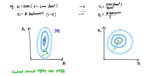
    losses.append(loss)

피쳐 스케일링

모든 feature가 비슷한 범위에 있으면 gradient descent가 더 빠르게 수렴하는 데에 도움이 된다.

방법들:
1) Standardization

$x' = \frac{x - \mu}{\sigma}$

평균을 뺀 후 표준편차로 나누기

$\mu$ = 평균
$\sigma$ = 표준편차

2) Min-Max Scaling

$x' = \frac{x - x_{min}}{x_{max} - x_{min}}$
결과: $0 \le x' \le 1$

3) Mean Normalization
$x' = \frac{x - \mu}{x_{max} - x_{min}}$
결과: -1 ~ 1

필요할 때

모델	필요성
Linear Regression	매우 중요
Logistic Regression	매우 중요
Neural Network	필수
SVM	매우 중요
KNN	매우 중요

안 필요할 때 (Tree 기반 모델)

모델
Random Forest
Decision Tree
XGBoost

예)

from sklearn.preprocessing import StandardScaler
scaler = StandardScaler()
X_scaled = scaler.fit_transform(X)