Lag-Llama: Towards Foundation Models for Probabilistic Time Series Forecasting
General purpose foundation model for univariate probabilistic time series forecasting
Use lags as covariates
Lag-Llama is pretrained on a large corpus of diverse time series data from several domains
1. Introduction
General purpose foundation model for univariate probabilistic time series forecasting
Statistical models
- Shortfall lies in their inherent assumption of linear relationships and stationarity
- May require extensive manual tuning and domain knowledge to select appropriate models and parameters
Foundation models
- Time-LLM, LLM4TS, GPT2 freeze LLM encoder backbones while simultaneously fine-tuning the input and distribution heads for forecasting
- Main goal of our work is to apply the foundation model approach to time series data
3. Probabilistic Time Series Forecasting
Univariate time series dataset
- Dtrain={x1:Tii}i=1D
- t∈{1,…,Ti}
- Ti : length of the time series i
- Predict the values at the future P
- Dtest={xTi+1:Ti+Pi}i=1D
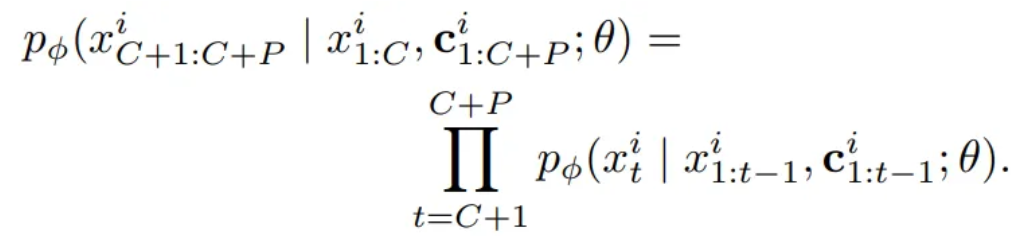
Univariate probabilistic time series forecasting problem
= Modelling an unknown joint distribution of the P future values
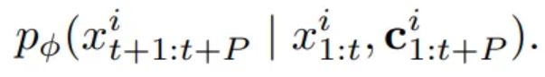
- ϕ : paramters of a parametric distribution
- Rather than considering the whole history of each time series i,
we can instead sub-sample fixed context windows of size C
Predictions are conditioned on these learned parameters θ
4. Lag-Llama
- When training on heterogenous univariate time series corpora, the frequency of the time series in our corpus varies
- When adapting model to downstream datasets, may encounter new frequencies and combinations of seen frequencies
→ General method for tokenizing series from such a dataset, without directly relying on the frequency of any specific dataset
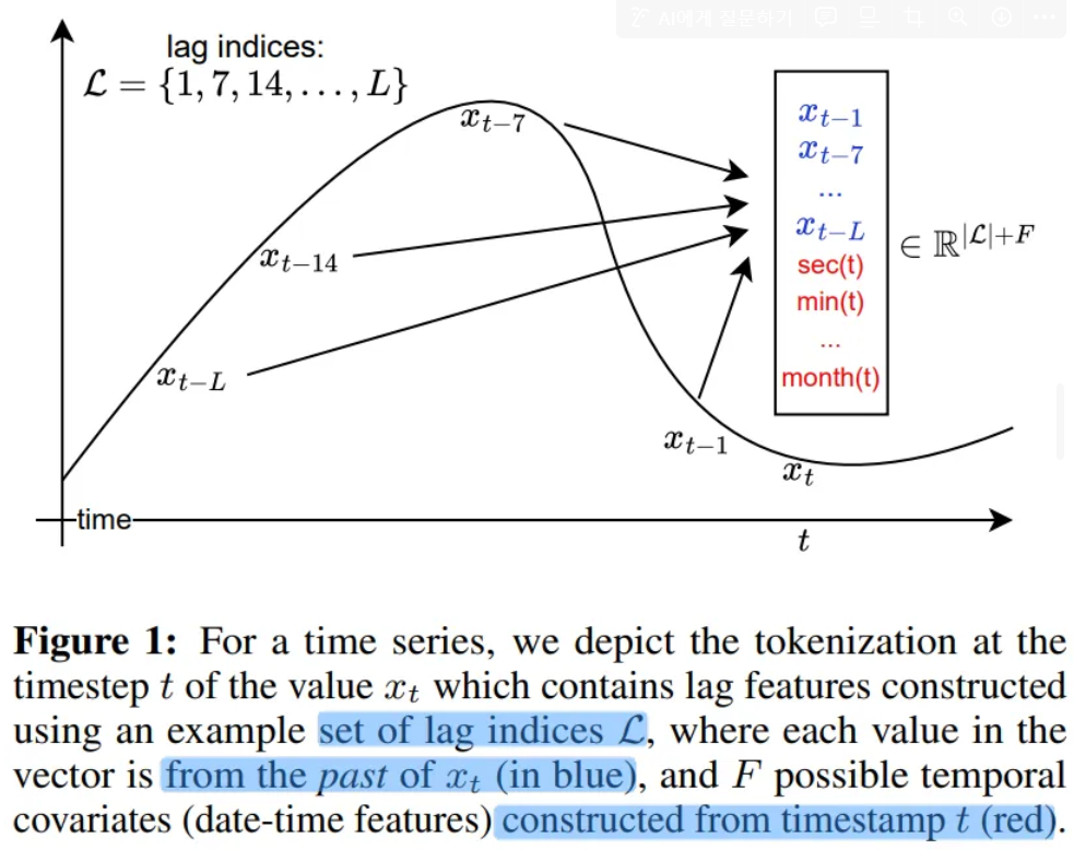
4.1. Tokenization : Lag Features
- Construct lagged features from the prior values of the time series
- Lag indices include quarterly, monthly, weekly, daily, hourly and second-level frequencies
To create lag features for some context-length window x1:C,
- Sample a larger window with L more historical points
- To these lagged features, add date-time features of all the frequencies
second of minute, hour of day etc. (Real time values of data) till the quarter of year from the time index t
- All except one date-time feature will remain constant from one time-step to the next and from the model can make sense of the frequency of the time series
- F : total of date time features
- → Each of tokens is of size £+F
4.2. Lag-Llama Architecture
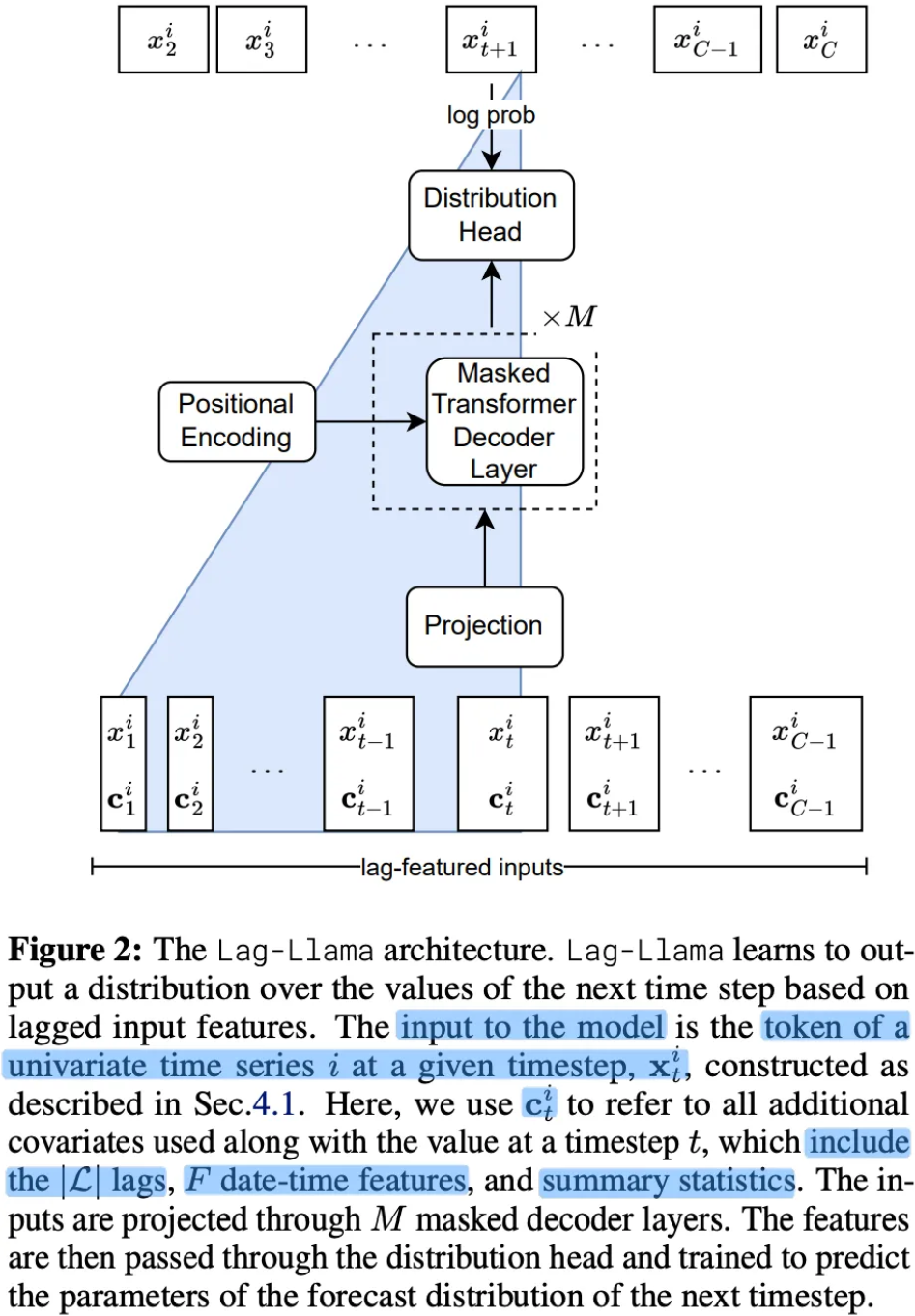
- A univariate sequence of length along with its covariates is tokenized by concatenating the covariates vectors to a sequence of C tokens
- Tokens are passed through a shared linear projection layer
- RMSNorm and Rotary Positional Encoding at each attention layer’s query and key representations
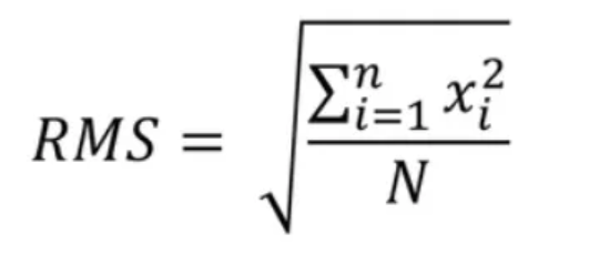
RMSNorm
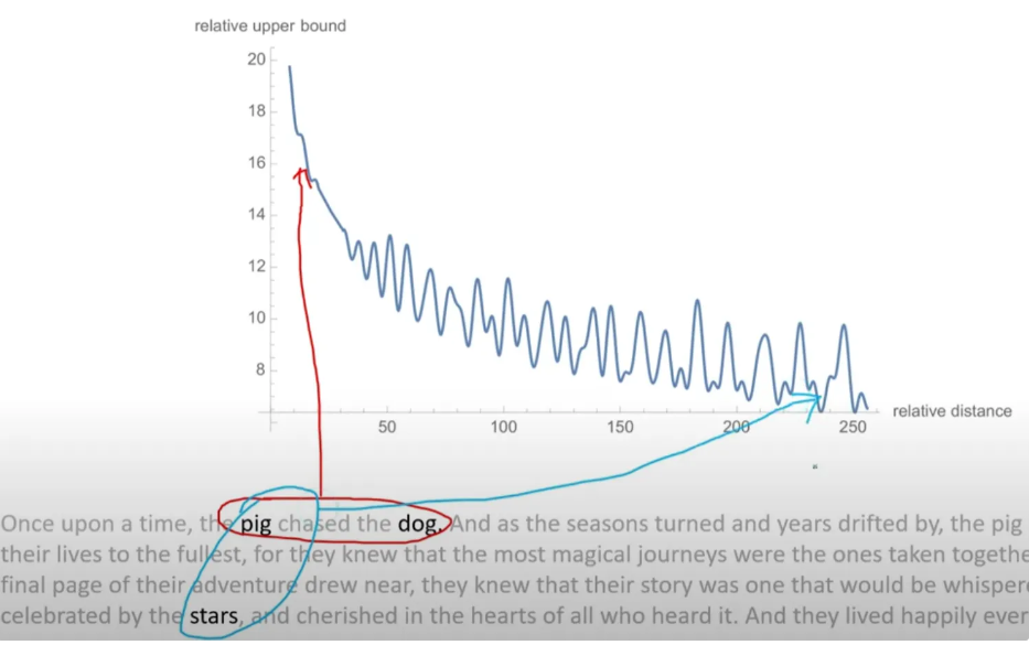
Rotary Positional Encoding
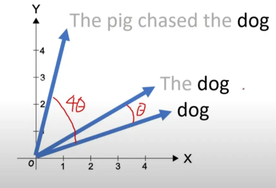
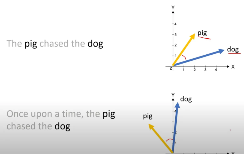
- As long as the distance between the two words stay same
- Multiply rotation matrix after Multiply query and key weight matrix
- Model predicts the parameters ϕ of the forecast distribution of the next timestep
- Parameters are output by a parametric distribution head
4.3. Choice of Distribution Head
- Last layer is the distribution head
which projects the model’s features to the parameters of a probability distribution
- Combine different distribution heads
- Adopt Student’s t-distribution and output the three parameters
Degrees of freedom, Mean, and Scale
- To ensure the parameters stay positive, appropriate non-linearity is used
4.4. Value Scaling
- Utilize the scaling heuristic
- For each univariate window, Calulate its mean and variance
- Scale x1:Ci → {(xti−μi)/σi}t=1C
- Also incorporate μi and σi as covariates for each token,
which we call summary statistics
- During training, values are transformed using the mean and variance,
while sampling, every timestep data is sampled is de-standardized
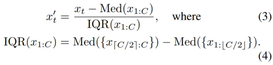
- In practice, instead of the standard scaler, Use Robust Standardization
Robust Standardization
4.5. Training Strategies
- Corpus are weighed by the amount of total number of series
- Augment with Freq-Mix and Freq-Mask
5. Experiment Setup
5.1. Datasets
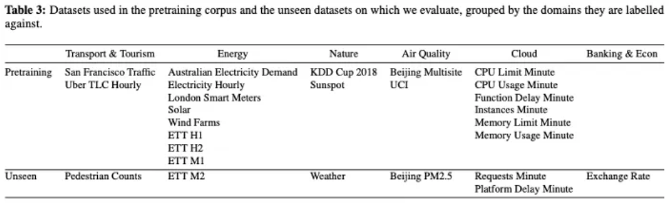
- Corpus of 27 time series datasets from six different domains
- Leave out a few datasets from each domain for testing the few-shot
- 7965 univariate time series
5.3. Model Training Setup
- Each epoch consists of 100 randomly sampled windows
- Since model is decoder-only and since prediction length is not fixed
the model can work for any downstream prediction length
6. Results
CRPS
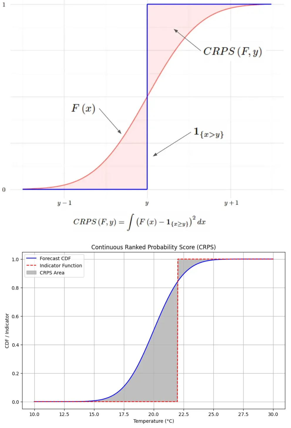
- μ=20,σ=2
- Observed value = 22
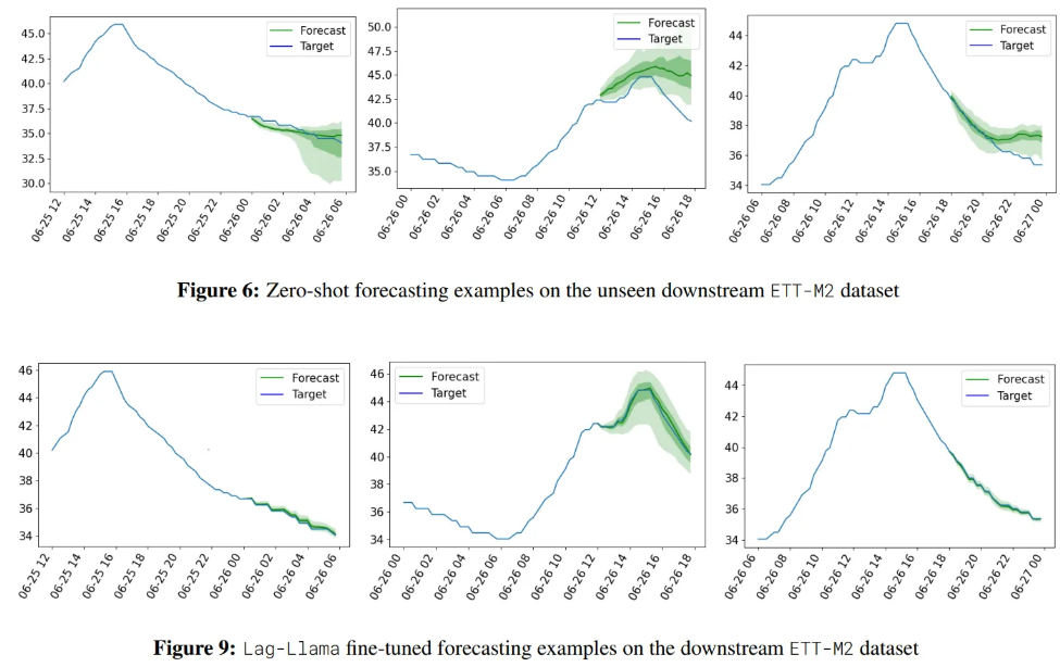
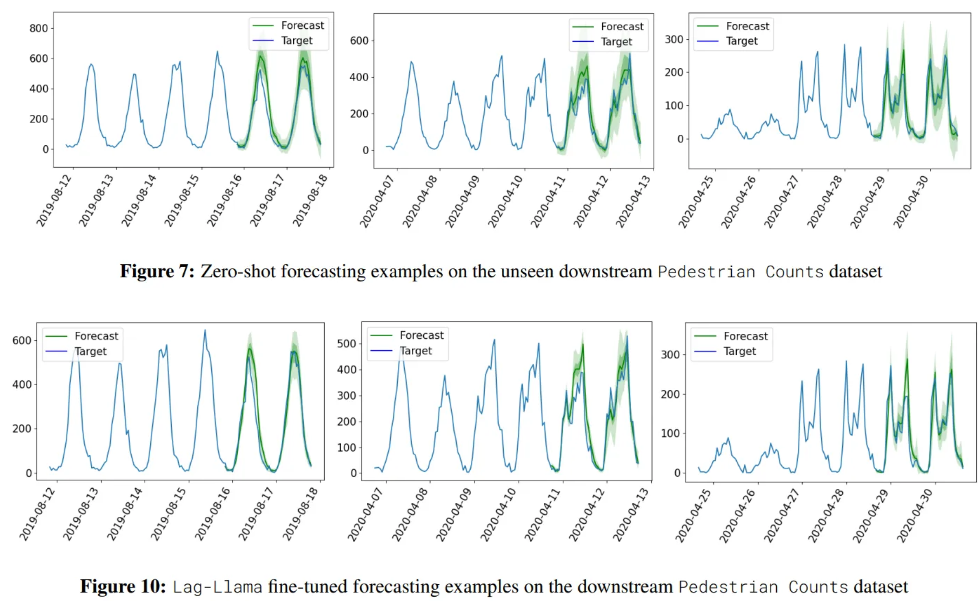
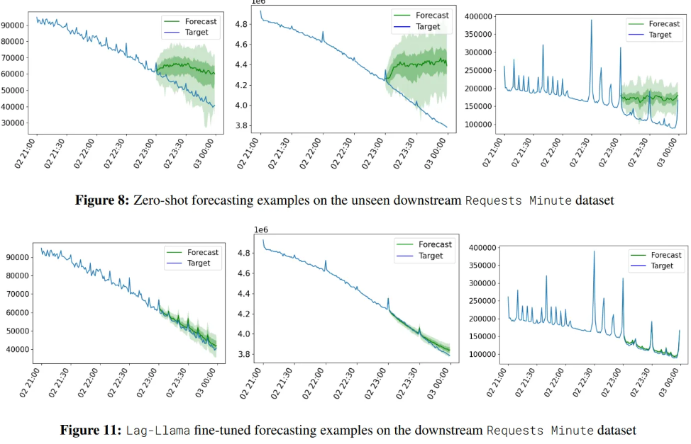
6.1. Zero-shot
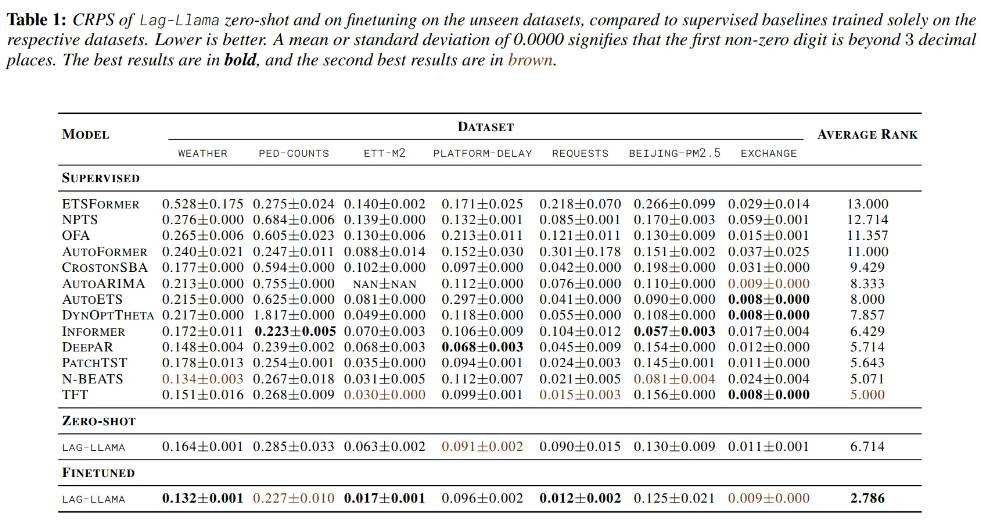
- Exchange-rate is an entirely new domain
- Inductive bias
- Vanilla decoder-only transformers outperform other transformer architectures
- As inductive bias gets larger, it performs well with smaller datasets
- Simple models with smaller inductive bias perform better when trained on large datasets.
- Compared to the OneFitsAll which adapts a pretrained LLM for forecasting, Lag-Llama achieves better performance
- Demonstrate the potential of foundation models trained from scratch compared to the adaptation of pretrained LLM
6.2. Few-shot
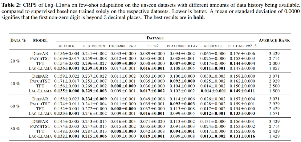
- Exchange-rate is entirely new domain and new unseen frequency
- most dissimilar as compared to the pretraining corpus
Visualization