03-06. 피마 인디언 당뇨병 예측

위키북스의 파이썬 머신러닝 완벽 가이드 책을 토대로 공부한 내용입니다.

1. Pima Indian Diabetes

피마 인디언 당뇨병 dataset을 이용하여 당뇨병 여부를 판단하는 ML 예측 모델을 만들고 평가 지표들을 적용시켜 볼 것이다.
피마 인디언 당뇨병 dataset의 feature 정보이다.

• Pregnancies : 임신 횟수
• Glucose : 포도당 부하 검사 수치
• BloodPressure : 혈압(nm Hg)
• SkinThickness : 팔 삼두근 뒤쪽의 피하지방 측정값(nm)
• Insulin : 혈청 인슐린(mu U/ml)
• BMI : 체질량지수(체중(kg)/(키(m))^2)
• DiabetesPedigreeFunction : 당뇨 내력 가중치 값
• Age : 나이
• Outcome : Class 결정 값(0 or 1)

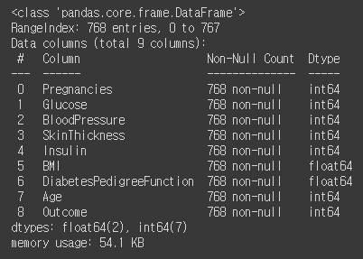
import pandas as pd

diabetes_data = pd.read_csv('/content/drive/MyDrive/pymldg-rev/3장/diabetes.csv')
print(diabetes_data['Outcome'].value_counts(), end='\n\n')
diabetes_data.info( )

[output] 전체 768개 data가 있으며 그 중 Negative가 500개, Positive가 268개로 Negative가 상대적으로 더 많다. Null 값은 없고 feature들은 모두 숫자형 data이다.

2. 모델 학습 / 평가 (1)

로지스틱 회귀를 이용햐 예측 모델을 생성하고, 이전의 get_clf_eval(), get_eval_by_threshold, precision_recall_curve_plot을 이용해 성능 평가를 해보았다.

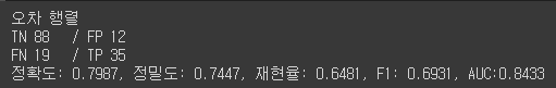
import numpy as np
import matplotlib.pyplot as plt
%matplotlib inline

from sklearn.model_selection import train_test_split
from sklearn.metrics import accuracy_score, precision_score, recall_score, roc_auc_score
from sklearn.metrics import f1_score, confusion_matrix, precision_recall_curve, roc_curve
from sklearn.preprocessing import StandardScaler
from sklearn.linear_model import LogisticRegression

# 수정된 get_clf_eval() 함수 
def get_clf_eval(y_test, pred=None, pred_proba=None):
    confusion = confusion_matrix( y_test, pred)
    accuracy = accuracy_score(y_test , pred)
    precision = precision_score(y_test , pred)
    recall = recall_score(y_test , pred)
    f1 = f1_score(y_test,pred)
    # ROC-AUC 추가 
    roc_auc = roc_auc_score(y_test, pred_proba)
    print('오차 행렬')
    print(f'TN {confusion[0][0]}\t/ FP {confusion[0][1]}')
    print(f'FN {confusion[1][0]}\t/ TP {confusion[1][1]}')
    # ROC-AUC print 추가
    print('정확도: {0:.4f}, 정밀도: {1:.4f}, 재현율: {2:.4f}, F1: {3:.4f}, AUC:{4:.4f}'.format(accuracy, precision, recall, f1, roc_auc))

def precision_recall_curve_plot(y_test , pred_proba_c1):
    # threshold ndarray와 이 threshold에 따른 정밀도, 재현율 ndarray 추출. 
    precisions, recalls, thresholds = precision_recall_curve( y_test, pred_proba_c1)

    # X축을 threshold값으로, Y축은 정밀도, 재현율 값으로 각각 Plot 수행. 정밀도는 점선으로 표시
    plt.figure(figsize=(8,6))
    threshold_boundary = thresholds.shape[0]
    plt.plot(thresholds, precisions[0:threshold_boundary], linestyle='--', label='precision')
    plt.plot(thresholds, recalls[0:threshold_boundary],label='recall')

    # threshold 값 X 축의 Scale을 0.1 단위로 변경
    start, end = plt.xlim()
    plt.xticks(np.round(np.arange(start, end, 0.1),2))

    # x축, y축 label과 legend, 그리고 grid 설정
    plt.xlabel('Threshold value'); plt.ylabel('Precision and Recall value')
    plt.legend(); plt.grid()
    plt.show()

# 피처 데이터 세트 X, 레이블 데이터 세트 y를 추출. 
# 맨 끝이 Outcome 컬럼으로 레이블 값임. 컬럼 위치 -1을 이용해 추출 
X = diabetes_data.iloc[:, :-1]
y = diabetes_data.iloc[:, -1]

X_train, X_test, y_train, y_test = train_test_split(X, y, test_size = 0.2, random_state = 156, stratify=y)

# 로지스틱 회귀로 학습,예측 및 평가 수행. 
lr_clf = LogisticRegression()
lr_clf.fit(X_train , y_train)
pred = lr_clf.predict(X_test)
pred_proba = lr_clf.predict_proba(X_test)[:, 1]

get_clf_eval(y_test , pred, pred_proba)

[output] 전체 데이터의 65%가 Negative이므로 정확도보다는 재현율 성능에 조금 더 초점을 맞춘다.

pred_proba_c1 = lr_clf.predict_proba(X_test)[:, 1]
precision_recall_curve_plot(y_test, pred_proba_c1)

[output] threshold가 0.42정도 일때 정밀도와 재현율이 어느정도 균형을 맞추는 듯 보이지만 2개의 지표가 모두 0.7도 안되는 수치를 보인다. 따라서 descrobe() method를 사용하여 다시 데이터의 분포를 점검한다.

3. 데이터 분석 / 전처리

diabetes_data.describe()

[output] 데이터 값을 확인해보면 min값이 0으로 되어 있는 feature들이 상당히 많다. 하지만 Glucose feature의 경우 포도당 수치를 의미하는 feature인데 min값이 0인 것은 말이 되지 않는다. 따라서 0값이 어느정도 존재하는지 자세하게 알기 위해 Glucose feature의 히스토그램을 확인해보았다.

plt.hist(diabetes_data['Glucose'], bins=10)

[output] 히스토그램을 보면 0값이 일정 수준 존재하는 것을 볼 수 있다. 따라서 전체 dataset 중 min값이 0으로 되어 있는 feature에 대해 0값이 어느정도 비율로 존재하는지 확인해보았다. 확인할 feature는 출산 횟수를 의미하는 Pregnancies를 제외한 Glucose, BloodPressure, SkinThickness, Insulin, BMI이다.

# 0값을 검사할 피처명 리스트 객체 설정
zero_features = ['Glucose', 'BloodPressure','SkinThickness','Insulin','BMI']

# 전체 데이터 건수
total_count = diabetes_data['Glucose'].count()

# 피처별로 반복 하면서 데이터 값이 0 인 데이터 건수 추출하고, 퍼센트 계산
for feature in zero_features:
    zero_count = diabetes_data[diabetes_data[feature] == 0][feature].count()
    print('{0} 0 건수는 {1}, 퍼센트는 {2:.2f} %'.format(feature, zero_count, 100*zero_count/total_count))

[output] 확인 결과를 보면 SkinThickness, Insulin의 0값은 상당히 높은 비율로 존재하는 것을 볼 수 있다. 하지만 전체 dataset 수가 많지 않은 상황이라 이 data들을 일괄적으로 삭제할 경우 학습을 효과적으로 수행하기 어려울것 같아 0값의 feature들을 평균값으로 대체하였다.

# zero_features 리스트 내부에 저장된 개별 피처들에 대해서 0값을 평균 값으로 대체
diabetes_data[zero_features]=diabetes_data[zero_features].replace(0, diabetes_data[zero_features].mean())

4. 모델 학습 / 평가 (2)

0값을 평균값으로 대체한 dataset에 feature scaling을 적용해 변환한 후 다시 학습/테스트 dataset을 나누고 로지스틱 회귀를 적용해 성능 평가 지표를 확인하였다.

from sklearn.preprocessing import StandardScaler

X = diabetes_data.iloc[:, :-1]
y = diabetes_data.iloc[:, -1]

# StandardScaler 클래스를 이용해 피처 데이터 세트에 일괄적으로 스케일링 적용
scaler = StandardScaler( )
X_scaled = scaler.fit_transform(X)

X_train, X_test, y_train, y_test = train_test_split(X_scaled, y, test_size = 0.2, random_state = 156, stratify=y)

# 로지스틱 회귀로 학습, 예측 및 평가 수행. 
lr_clf = LogisticRegression()
lr_clf.fit(X_train , y_train)
pred = lr_clf.predict(X_test)
pred_proba = lr_clf.predict_proba(X_test)[:, 1]

get_clf_eval(y_test , pred, pred_proba)

[output] 데이터 변환과 스케일링을 통해 어느 정도 성능이 개선되었다. 하지만 재현율은 아직 작은 값을 보이고 있어 분류 결정 threshold를 변화시키며 재현율의 성능이 얼마나 개선되는지 확인해보았다.

from sklearn.preprocessing import Binarizer

def get_eval_by_threshold(y_test , pred_proba_c1, thresholds):
    # thresholds 리스트 객체내의 값을 차례로 iteration하면서 Evaluation 수행.
    for custom_threshold in thresholds:
        binarizer = Binarizer(threshold=custom_threshold).fit(pred_proba_c1) 
        custom_predict = binarizer.transform(pred_proba_c1)
        print('임곗값:',custom_threshold)
        print('-'*80)
        get_clf_eval(y_test , custom_predict, pred_proba_c1)
        print('='*80)
      
thresholds = [0.3, 0.33, 0.36, 0.39, 0.42, 0.45, 0.48, 0.50]
pred_proba = lr_clf.predict_proba(X_test)
get_eval_by_threshold(y_test, pred_proba[:,1].reshape(-1,1), thresholds)

[output] 위 결과에 따르면 전체적인 성능 지표를 유지하면서 재현율을 약간 향상시키는 좋은 threshold는 0.48로 보인다. 따라서 학습된 로지스틱 회귀 모델을 이용해 threshold 0.48로 다시 예측을 해보겠다.

# 임곗값를 0.48로 설정한 Binarizer 생성
binarizer = Binarizer(threshold=0.48)

# 위에서 구한 lr_clf의 predict_proba() 예측 확률 array에서 1에 해당하는 컬럼값을 Binarizer변환. 
pred_th_048 = binarizer.fit_transform(pred_proba[:, 1].reshape(-1,1)) 
get_clf_eval(y_test , pred_th_048, pred_proba[:, 1])

[output]