Paint Transformer: Feed Forward Neural Painting with Stroke Prediction

Abstract

• Neural Painting: Neural Network로 주어진 이미지를 기반으로 사진 같지 않은 이미지를 stroke의 series로 재창조하는 것
• 이전 방법
  • Reinforcement learning 기반 agent가 이 task를 할 수 있지만 학습시키기가 어려움
  • Stroke optimization 기법은 stroke parameter의 집합을 찾는 방법을 찾음
    • 효율이 낮음
• Paint transformer: 논문에서는 set prediction problem을 만들었고, transformer 기반의 framework를 제안함
  • Feed forward network로 stroke set parameter를 예측함
  • 거의 실시간으로 512x512 final painting 생성 가능
  • Self-training pipeline 만듦, off-the-shelf dataset 필요 없음

Introduction

• 이미지 변환 모델들: pixel 단위로 처리하는 방식
  • Image style transfer
  • Image-to-image translation
• 사람은 stroke-to-stroke로 그림을 그림 -> 이걸 만들어보자
• stroke-to-stroke를 위한 시도들, efficiency와 effectiveness에서 개선할 부분이 많이 남음
  • RNN
  • Step-wise greedy search
  • Reinforcement learning: 학습 시간 김
  • Iterative optimization process: 학습 x, 하지만 처리 시간 엄청 김
• 논문에서는 stroke sequence generation 대신에 feed-forward stroke set prediction problem으로 재정의하여 해걸
• initial canvas와 target natural image 차이를 최소화하는 set of stroke 예측
  • 큰 stroke부터 작은 stroke 까지(coarse-to-fine) K scale을 따라 진행
• robust stroke set predictor를 학습하는 게 핵심 문제
  • object detection 문제와 유사함
• DETR로부터 영감 얻음
• parameters of multiple strokes with a feed forward Transformer
• object detection과 차이점: annotated data가 없음 -> self-training pipeline 제안, synthesized stroke image 활용
• Pipeline
  • 배경 canvas image를 임의의 sample stroke로 합성
  • 임의의 전경 stroke set을 뽑아서, target image와 가까워지도록 render 함
• stroke predictor의 목적은 synthesized canvas image와 target image의 차이를 최소화하는 것
• stroke level과 pixel level 각각 최적화 수행
• 한 번 학습되면 어떤 이미지든 활용 가능
• 주요 contributions
  • 문제 정의 변경: stroke-based neural painting problem -> feed-forward stroke set prediction
  • self-training strategy
  • quality, efficiency 좋음

2. Related Works

2.2. Object Detection

• DETR을 선택한 이유: post-processing이 없어서
• 우리는 DETR에 binary neurons를 추가함, 대신에 input으로 2개의 이미지를 넣음

3. Methods

3.1 Overall Framework

• neural painting을 progressive stroke prediction process로 정의함
• Paint Transformer의 modules
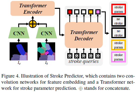
  • Stroke Predictor
  • Stroke Renderer

• Fig. 2 process
  • target image $I_t$와 intermediate canvas image $I_c$가 주어짐
  • ??
• Stroke Predictor만 trainable parameter를 가짐
• Stroke Renderer는 미분 가능하며 parameter 없음
• 학습을 위해 randomly synthesized strokes 활용
• 학습 iteration의 process
  • foreground stroke set $S_f$를 뽑고, background stroke $S_b$를 뽑음
    • 어떻게?
  • $S_b$ 넣어서 canvas image $I_c$ 출력
  • $I_c$ 위에 $S_f$를 render 하여 $I_t$ 출력
  • $I_c$, $I_t$를 넣어서 $S_r$ 출력
  • $S_r$, $I_c$ 넣어서 $I_r$ 출력

• Stroke Predictor의 objective function

  $\mathcal{L} = \mathcal{L}_{stroke}(S_r, S_f) + \mathcal{L}(I_r, I_t)$

• supervision을 위한 strokes는 임의로 합성되기 때문에 off-the-shelf-dataset 필요없음

3.2 Stroke Definition and Renderer

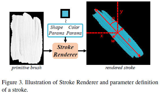
Parameters: $\{x,y,h,w,\theta,r,g,b\}$

• end-to-end training을 위해 미분 가능해야 함

• Stroke Renderer

  $I_{out} = StrokeRenderer(I_{in}, S)$

• alpha map -> 이해 안됨

3.3 Stroke Predictor

• intermediate canvas image와 target image의 차이를 줄이는 set of strokes를 예측하는 것이 목적
• 가능하면 적은 수의 stroke로 예측하도록 함
  $S_r = StrokePredictor(I_c, I_t)$
  

$I_c, I_t \in R^{3\times P \times P}$ -> $F_c, F_t \in R^{C \times P/4 \times P/4}$

• Transformer encoder에 입력되는 것
  • $F_c, F_t$
  • Learnable positional encoding
• Transformer decoder에 입력되는 것
  • N learnable stroke query vectors
• Transforemr decoder가 출력하는 것
  • Initial stroke parameters: $S_r = \{s_i\}^{N}_{i=1}$
  • Stroke confidence: $C_r = \{c_i\}^{N}_{i=1}$
    • Stroke confidence에 binary neurons를 추가함
      • Forward phase 일 때, $d_i = Sign(c_i)$, -> $c_i >0$ 이면 $d_i =1$, 아니면 $d_i=0$
      • $d_i$는 stroke를 canvas에 그릴지 말지를 결정함
      • backward phase 일 때,Sigmoid 사용
        $\frac{\partial d_i}{\partial c_i} = \frac{\partial \sigma (c_i)}{\partial c_i} = \frac{\exp(-c_i)}{(1+\exp(-c_i))^2}$

3.4 Loss Function

Pixel Loss

Stroke Distance

• L1 distance
  $\mathcal{D}^{u,v}_{L_1} = ||s_u - s_v||_1$
• L1 distance는 big, small strokes 간 scale 차이를 무시함 -> Wasserstein distance 추가
• 2D Gaussian Distribution $\mathcal{N}(\mu, \Sigma)$
• Wasserstein distance between two Gaussian distributions
  $\mathcal{D}_W^{u,v} = ||\mu_u - \mu_v||^2_2 + Tr(\Sigma_u + \Sigma_v - 2(\Sigma_u^{\frac{1}{2}} \Sigma_v \Sigma_u^{\frac{1}{2}})^{\frac{1}{2}})$

Stroke Loss

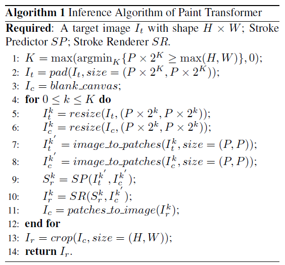
3.5 Inference