
Linear Regression with Gradient Descent
Linear regression with one variable, implemented by numpy
import matplotlib.pyplot as plt
%matplotlib inline
import pandas as pd
import numpy as np
LOAD DATASET
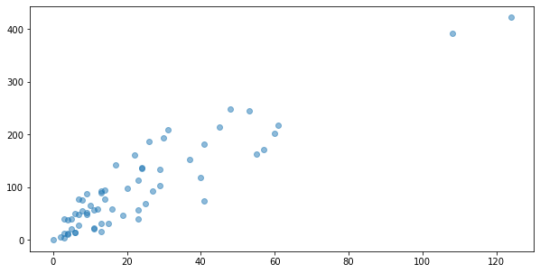
In the following data
- X = number of claims
- Y = total payment for all the claims in thousands of Swedish Kronor
for geographical zones in Sweden Reference: Swedish Committee on Analysis of Risk Premium in Motor Insurance
dataset from - http://college.cengage.com/mathematics/brase/understandable_statistics/7e/students/datasets/slr/frames/frame.html
df = pd.read_csv("slr06.csv")
df.head()| X | Y | |
|---|---|---|
| 0 | 108 | 392.5 |
| 1 | 19 | 46.2 |
| 2 | 13 | 15.7 |
| 3 | 124 | 422.2 |
| 4 | 40 | 119.4 |
raw_X = df["X"].values.reshape(-1, 1)
y = df["Y"].valuesplt.figure(figsize=(10,5))
plt.plot(raw_X,y, 'o', alpha=0.5)[<matplotlib.lines.Line2D at 0x1b548d68040>]
raw_X[:5], y[:5] (array([[108],
[ 19],
[ 13],
[124],
[ 40]], dtype=int64),
array([392.5, 46.2, 15.7, 422.2, 119.4]))
np.ones((len(raw_X),1))[:3] array([[1.],
[1.],
[1.]])
X = np.concatenate( (np.ones((len(raw_X),1)), raw_X ), axis=1)
X[:5]
array([[ 1., 108.],
[ 1., 19.],
[ 1., 13.],
[ 1., 124.],
[ 1., 40.]])
w = np.random.normal((2,1))
# w = np.array([5,3])
w
array([2.71493328, 0.01260081])
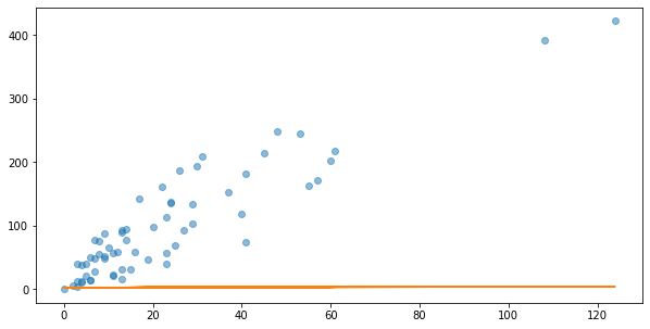
plt.figure(figsize=(10,5))
y_predict = np.dot(X, w)
plt.plot(raw_X,y,"o", alpha=0.5)  #alpha=learning rate
plt.plot(raw_X,y_predict)
[<matplotlib.lines.Line2D at 0x1b548e4f130>]
HYPOTHESIS AND COST FUNCTION
def hypothesis_function(X, theta):
    return X.dot(theta)
h = hypothesis_function(X,w)def cost_function(h, y):
return (1/(2*len(y))) * np.sum((h-y)**2)h = hypothesis_function(X,w)
cost_function(h, y)8259.456440618966
GRADIENT DESCENT
def gradient_descent(X, y, w, alpha, iterations):
    theta = w
    m = len(y)

    theta_list = [theta.tolist()]
    cost = cost_function(hypothesis_function(X, theta), y)
    cost_list = [cost]

    for i in range(iterations):
        t0 = theta[0] - (alpha / m) * np.sum(np.dot(X, theta) - y)
        t1 = theta[1] - (alpha / m) * np.sum((np.dot(X, theta) - y) * X[:,1])
        theta = np.array([t0, t1])

        if i % 10== 0:  #변화 확인을 위해 10번마다 theta list와 cost list 반환
            theta_list.append(theta.tolist())
            cost = cost_function(hypothesis_function(X, theta), y)
            cost_list.append(cost)


    return theta, theta_list, cost_list
DO Linear regression with GD
iterations = 10000
alpha = 0.001

theta, theta_list, cost_list = gradient_descent(X, y, w, alpha, iterations)
cost = cost_function(hypothesis_function(X, theta), y)

print("theta:", theta)
print('cost:', cost_function(hypothesis_function(X, theta), y))
theta: [19.88487261 3.41619037]
cost: 625.3740024992405
theta_list[:10] [[2.714933281281911, 0.012600813595122662],
[2.810117030952728, 4.018053960854277],
[2.891767860497031, 3.7831117980615105],
[2.9780141038123125, 3.78124953713786],
[3.0638254212561615, 3.779396667295376],
[3.149204006089478, 3.7775531411761647],
[3.2341520405129063, 3.7757189116613405],
[3.318671695722605, 3.7738939318696283],
[3.4027651319657433, 3.7720781551561693],
[3.48643449859571, 3.770271535111326]]
theta_list = np.array(theta_list)cost_list[:5] [8259.456440618966,
728.9295257860615,
699.3255878015307,
698.5815860507722,
697.8450691411475]
plt.figure(figsize=(10,5))

y_predict_step= np.dot(X, theta_list.transpose())

y_predict_step
plt.plot(raw_X,y,"o", alpha=0.5)
for i in range (0,len(cost_list),100):
    plt.plot(raw_X,y_predict_step[:,i], label='Line %d'%i)

plt.legend(bbox_to_anchor=(1.05, 1), loc=2, borderaxespad=0.)
plt.show()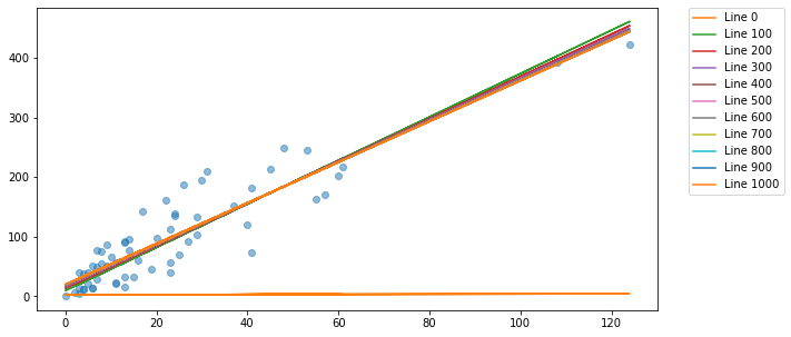
plt.plot(range(len(cost_list)), cost_list);
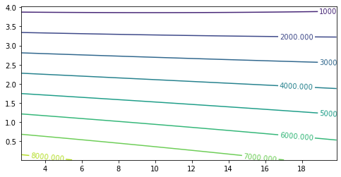
th0 = theta_list[:,0]
th1 = theta_list[:,1]
TH0, TH1 = np.meshgrid(th0, th1)
Js = np.array([cost_function(y, hypothesis_function(X, [th0, th1])) for th0, th1 in zip(np.ravel(TH0), np.ravel(TH1))])
Js = Js.reshape(TH0.shape)plt.figure(figsize=(8,4))
CS = plt.contour(TH0, TH1, Js)
plt.clabel(CS, inline=True, fontsize=10,inline_spacing=2)<a list of 8 text.Text objects>
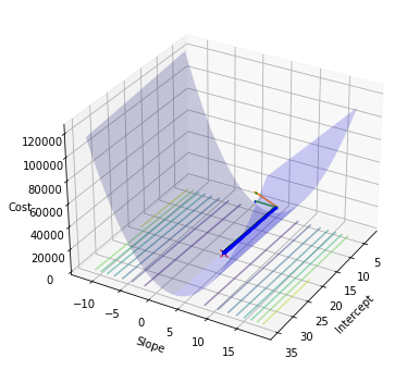
from mpl_toolkits.mplot3d import Axes3D

ms = np.linspace(theta[0] - 15 , theta[0] + 15, 100)
bs = np.linspace(theta[1] - 15 , theta[1] + 15, 100)

M, B = np.meshgrid(ms, bs)

zs = np.array([ cost_function(y, hypothesis_function(X, theta))
    for theta in zip(np.ravel(M), np.ravel(B))])
Z = zs.reshape(M.shape)
fig = plt.figure(figsize=(10, 6))
ax = fig.add_subplot(111, projection='3d')
ax.plot_surface(M, B, Z, rstride=1, cstride=1, color='b', alpha=0.2)
ax.contour(M, B, Z, 10, color='b', alpha=0.5, offset=0, stride=30)
ax.set_xlabel('Intercept')
ax.set_ylabel('Slope')
ax.set_zlabel('Cost')
ax.view_init(elev=30., azim=30)
ax.plot([theta[0]], [theta[1]], [cost_list[-1]] , markerfacecolor='r', markeredgecolor='r', marker='x', markersize=7);
ax.plot(theta_list[:,0], theta_list[:,1], cost_list, markerfacecolor='g', markeredgecolor='g', marker='o',
markersize=1);
ax.plot(theta_list[:,0], theta_list[:,1], 0 , markerfacecolor='b', markeredgecolor='b', marker='.', markersize=2); :5: UserWarning: The following kwargs were not used by contour: 'color'
ax.contour(M, B, Z, 10, color='b', alpha=0.5, offset=0, stride=30)
https://www.boostcourse.org/ai222/lecture/253410
https://www.boostcourse.org/ai222/lecture/253411