Evaluation Metrics for Classification

분류문제의 평가지표

1. 정확도(Accuracy) : 옳게 맞춘 것을 전체 수로 나눈 값
   $\large \frac{TP + TN}{Total}$

2. 정밀도(Precision) : Positive로 예측한 경우 중 올바르게 Positive를 맞춘 비율
   $\large \frac{TP}{TP + FP}$

3. 재현율(Recall, Sensitivity) : 실제 Positive인 것 중 올바르게 Positive를 맞춘 것의 비율
   $\large \frac{TP}{TP + FN}$

4. F1점수(F1 score) : 정밀도와 재현율의 조화평균(harmonic mean)
   $2\cdot\large\frac{precision\cdot recall}{precision + recall}$

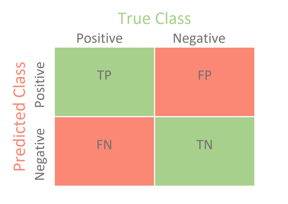
• True Positive(TP) : True라고 예측한 것이 정말로 True인 경우
• True Negative(TN) : False라고 예측한 것이 정말로 False인 경우
• False Positive(FP) : True라고 예측한 것이 사실은 False인 경우
• False Negative(FN) : False라고 예측한 것이 사실은 True인 경우

Confusion Matrix

분류 모델의 성능 평가 지표

from sklearn.metrics import plot_confusion_matrix
import matplotlib.pyplot as plt

pipe = make_pipeline(
    OrdinalEncoder(), 
    SimpleImputer(), 
    RandomForestClassifier(n_estimators=100, random_state=2, n_jobs=-1)
)

# 시각화
fig, ax = plt.subplots()
pcm = plot_confusion_matrix(pipe, X_val, y_val,
                            cmap=plt.cm.Blues,
                            ax=ax);
plt.title(f'Confusion matrix, n = {len(y_val)}', fontsize=15)
plt.show()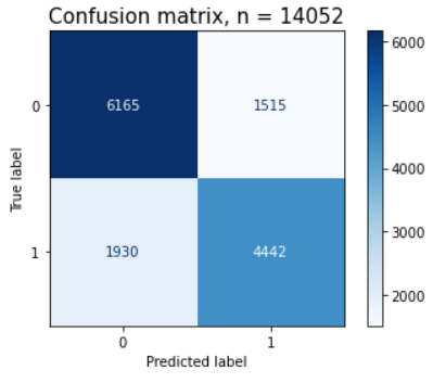

pcm.confusion_matrix
# 출력
array([[6165, 1515],
       [1930, 4442]])
       
# 정밀도, 재현율 확인
from sklearn.metrics import classification_report
print(classification_report(y_val, y_pred))
# 출력
                precision    recall  f1-score   support

           0       0.76      0.80      0.78      7680
           1       0.75      0.70      0.72      6372

    accuracy                           0.75     14052
   macro avg       0.75      0.75      0.75     14052
weighted avg       0.75      0.75      0.75     14052

---

임계값

from sklearn.pipeline import make_pipeline
from category_encoders import OrdinalEncoder
from sklearn.impute import SimpleImputer
from sklearn.ensemble import RandomForestClassifier
from sklearn.metrics import accuracy_score

pipe = make_pipeline(
    OrdinalEncoder(), 
    SimpleImputer(), 
    RandomForestClassifier(n_estimators=100, random_state=2, n_jobs=-1)
)
# 검증세트로 확률예측
pipe.predict_proba(X_val)
# 출력
array([[0.46      , 0.54      ],
       [0.85      , 0.15      ],
       [0.78      , 0.22      ],
       ...
       0일확률       1일확률

※ 임계값을 0.7를 하면 1일확률이 0.7이 넘는 쪽으로 분류한다
ex) [0.46, 0.54]면 0   /   [0.15, 0.85]면 1
임계값을 낮추면 정밀도는 올라가고 재현율은 떨어진다

※어떤 경우 필요한가?
ex) 임계값을 낮추어 백신을 접종하지 않을 확률이 높은 사람들을 더 정확하게 구하는 것이 도움이 된다

ROC curve, AUC

ROC curve는 여러 임계값에 대한 TPR(True Positive Rate, recall)과 FPR(False Positive Rate) 그래프

• Recall(재현율) : ${\frac {\mathrm {TP} }{\mathrm {TP} +\mathrm {FN} }}$
• Fall-out(위양성률) : ${\frac {\mathrm {FP} }{\mathrm {FP} +\mathrm {TN} }}$

• 재현율을 높이기 위해서는 Positive로 판단하는 임계값을 계속 낮추어 모두 Positive로 판단하게 만들면 된다. 하지만 이렇게 하면 동시에 Negative이지만 Positive로 판단하는 위양성률도 같이 높아진다
• 재현율은 최대화 하고 위양성률은 최소화 하는 임계값이 최적의 임계값
• AUC 는 ROC curve의 아래 면적

from sklearn.metrics import roc_curve

y_pred_proba = pipe.predict_proba(X_val)[:, 1]
fpr, tpr, thresholds = roc_curve(y_val, y_pred_proba)

roc = pd.DataFrame({
    'FPR(Fall-out)': fpr, 
    'TPRate(Recall)': tpr, 
    'Threshold': thresholds
})
# ROC curve 시각화
plt.scatter(fpr, tpr)
plt.title('ROC curve')
plt.xlabel('FPR(Fall-out)')  # x축
plt.ylabel('TPR(Recall)');   # y축

optimal_idx = np.argmax(tpr - fpr)
optimal_threshold = thresholds[optimal_idx]  # 최적 임계값
print('idx:', optimal_idx, ', threshold:', optimal_threshold)  # 출력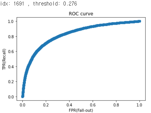

# AUC 점수
from sklearn.metrics import roc_auc_score
auc_score = roc_auc_score(y_val, y_pred_proba)
auc_score
# 출력
0.82653190

# 테스트세트로 에측 
y_test_proba = pipe.predict_proba(X_test)[:, 1]
y_test_optimal = y_test_proba >= optimal_threshold  #임계값보다 높은 것
# 제출 form
submission = pd.DataFrame(y_test_optimal).reset_index().astype(int)