설명
RANSAC이란
-
RANSAC은 RANdom SAmple Consensus의 줄임말로, 데이터를 랜덤하게 샘플링하여 사용하고자 하는 모델을 맞춘(
fitting) 다음 그 결과가 원하는 목표치(합의점,Consensus)에 도달하였는지 확인하는 과정을 통해 모델을 데이터에 맞게 최적화하는 과정이다.- 즉, 목표치가 최대인, 가장 많은 수의 데이터를 포함하는 모델을 선택하는 방법이다.
-
데이터에서 노이즈를 제거하고 모델을 예측하는 알고리즘으로, 특히 컴퓨터 비전 분야에서 광범위하게 사용된다.
-
선형, 다항 함수, 비선형 함수 등 어떤 모델이든 상관없이
모델 fitting과정을 적용할 수 있다. -
특정 임계값(
threshold) 이상의 데이터를 완전히 무시하는 특성이 있어outlier, 즉 정상 분포 밖의 이상값에 강건한(Robust) 알고리즘이다.Inlier: 데이터의 분포에 포함된 정상적인 관측값.
Outlier: 데이터의 분포에서 현저하게 벗어나 있는 관측값. 이상치와는 개념적으로 다르나, 실용적으로는 구분하기 힘들다.
-
아래 그래프를 통해 최소자승법과 RANSAC의 강건함을 비교할 수 있다.
- 원본 값과 최소자승법 적용 결과
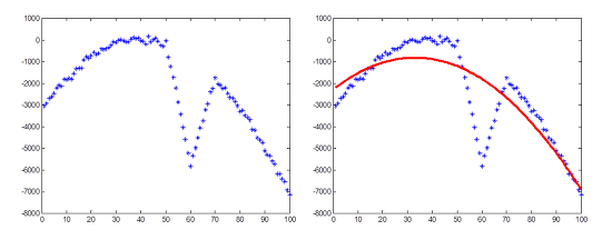
- RANSAC 적용 결과
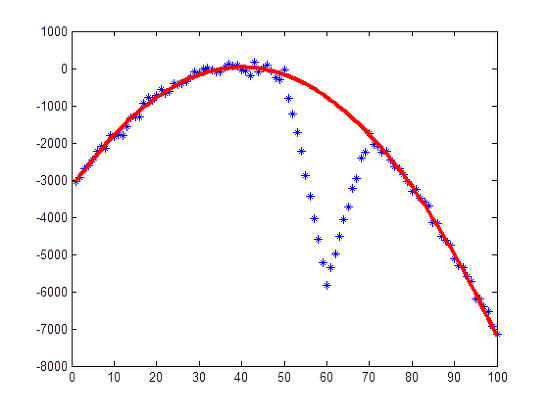
- 원본 값과 최소자승법 적용 결과
순서
-
RANSAC은 가설 단계와 검증 단계를 반복하는 것으로 최적의 모델을 구한다.
-
가설 단계에서 N개의 샘플을 선택하고, 샘플을 바탕으로 모델을 예측한다.
-
검증 단계에서 전체 데이터에서 예측 모델과 일치하는 데이터 수를 세어 목표치가 더 높다면 새롭게 모델을 저장한다.
-
이를 N번 반복하여 그 중 최적의 모델을 출력한다.
-
-
아래는 그 과정의 흐름도와 그 설명이다.

Pick n random points:inlier와outlier가 섞여 있는 전체 데이터셋에서 n개의 데이터 (포인트)를 랜덤 샘플링한다.Estimate model parameters: 랜덤 샘플 데이터를 이용하여 사용하고자 하는 모델을fitting한다.Calculate distance error: ② 과정을 통해fitting한 모델과 전체 데이터에 대하여error(차이)를 구한다.Count number of inliers: ③ 과정에서 구한error를 통해 각 데이터가inlier인 지outlier인 지 판단한다. 이 때 판단하는 근거는threshold기준을 정하여 판단합니다.threshold가 크면 많은 실제outlier또한inlier가 될 수 있으며, 반대로 작으면 많은 반복이 필요해질 수 있으므로 적당한 수준으로 정해야 한다.Maximum Inliers ?:inlier목표치 또는inlier데이터 비율의 목표치가 있고 현재fitting한 모델이 이 목표치를 달성하였다면iteration(반복 과정)을 끝낼 수 있다.(후에 설명할early stop전략이다.) 만약 목표치를 달성하지 못하였다면 앞선 과정을 반복한다.N iterations ?: 위 flow-chart를 통해 최대 N번의iteration을 반복하여RANSAC을 진행한다. N이 커질수록 시도할 수 있는 횟수가 많아지기 때문에 좋은 모델을 선택할 수 있는 가능성이 커지지만, 그만큼 수행시간이 늘어나게 된다.
-
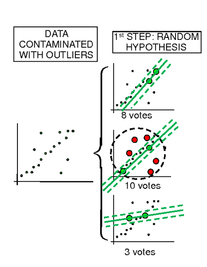
아래 그림 예시를 보면, 왼쪽의 원본 데이터셋에 대하여 랜덤으로 데이터를 2개씩 추출한 후, 샘플을 통해 모델을 예측한 그림이다.
-
초록색 실선이 모델, 점선이 임계값의 영역이다. 점선 내부가
inlier로 판단되고, 이inlier수가 많을수록 목표치가 높다고 판단한다. -
이 과정을 반복해 그 중 가장 목표치가 높은 최적의 모델을 찾는 것이다.
-
Early Stop 전략
-
RANSAC을 통해 반복적으로 모델을 최적화 할 때, 적합한 모델을 찾았다면 더 이상 모델 fitting 작업을 할 필요가 없다. 따라서 다음과 같이 3가지 파라미터를 정하여 RANSAC을 일찍 끝내는
Early Stop전략을 사용할 수 있다.-
min iteration: 최소 반복 횟수. -
max iteration: 최대 반복 횟수. 이만큼 반복하면 모델 fitting이 실패했다는 뜻이다. -
stop inlier ratio: 반복 작업을 끝내기 위한 최소inlier의 비율이다. 전체 데이터 기준inlier비율이 해당 값을 초과하면 RANSAC 작업을 종료한다.
-
RANSAC의 파라미터 설정
-
RANSAC에서 데이터를 추출했을 때 현재 추출된 샘플이 모두
inlier인지 아닌지는 판별할 수 없다. 그저 일치하는 데이터가 더 많은가 적은가를 판단할 수 있을 뿐이다. -
같은 이유로 RANSAC은 기존보다 더 개선된 모델인지만 판단할 수 있을 뿐 이것이 최고의 모델인지는 아무도 알 수 없다.
-
하지만 우리는 유한시간 내에서 RANSAC알고리즘을 완료해야하기 때문에 종료 시점, 즉 반복 횟수를 정해야 한다. 이를 이라고 한다.
=
inlier로만 이루어진 샘플을 획득할 확률 – 샘플링 성공=
dataset에서inlier의 비율= 회당 추출하는 데이터 수
= 알고리즘 반복 회수
-
데이터를 분석하는 입장에서 정할 수 있는 값은 이다. 은 작을수록, 은 클수록 구하는 샘플의 확률 가 커진다.
-
이 클수록 샘플링 해야 하는 데이터의 수가 많아지기 때문에
**outlier가 선택될 가능성이 더 커지게 된다.** 즉inlier로만 이루어진 샘플을 얻을 확률이 낮아지므로 가 작아진다.- 이러한 이유로 모델링에 필요한 최소 갯수를 샘플링 하는 방법을 많이 사용한다. 예를 들면 선형 모델을 모델링할 때에는 2개의 샘플만 있으면 되기 때문에 가 될 수 있다. 2차 함수 모델의 경우 3개의 샘플이 필요하므로 이 된다. 따라서 RANSAC에 사용되는 모델에 따라서 은 자동으로 결정될 수 있다.
-
따라서 바라는 가 있다면 바뀌는 건 뿐이다.
- 예를 들어, 위 포물선 근사 예에서
inlier비율이 80%라고 했을 때, RANSAC 성공확률을 99.9%로 맞추려면 필요한 반복 횟수는 다음과 같이 계산된다.
- 수학적 확률로 RANSAC을 10번만 돌려도 99.9% 확률로 해(반복 횟수)를 찾을 수 있다는 얘기이다. 생각보다 숫자가 작아서 를 99.99%로 놓고 계산해 봐도 이 나온다.
- 예를 들어, 위 포물선 근사 예에서
-
그리고 만큼 중요한 파라미터가
threshold, 즉 임계값인 이다. 모델을 예측하고, 데이터가 이 모델에 일치하는지 아닌지 판별할 때 모델과 데이터의 차이가 보다 작으면inlier, 크면outlier로 구분하게된다.-
를 너무 크게하면 모델간의 변별력이 없어지고 를 너무 작게하면 RANSAC 알고리즘이 불안정해진다.
-
를 선택하는 가장 좋은(일반적인) 방법은
inlier들의 잔차 분산을 이라 할때, 또는 정도로 잡는 것이다. -
먼저 RANSAC을 적용하고자 하는 실제 문제에 대해서
inlier들로만 구성된 실험 데이터들을 획득하고,inlier데이터들에 대해서 최소자승법을 적용하여 가장 잘 근사되는 모델을 구한다. -
이 모델과
inlier들과의 잔차를 구한 후 분산을 구해, 그 표준편차 를 구해서 이에 비례하게 를 결정한다. 잔차가 정규분포를 따른다면, 로 잡으면 97.7%, 로 잡으면 99.9%의 inlier들을 포함한다.
-
장단점
장점
-
outlier에 강건한(robust) 모델을 출력한다.outlier을 어느 정도 무시하고 모델링할 수 있다.
-
outlier에 강건한(robust) 모델을 설계하는 가장 쉬운 방법이다.inlier의 개수만 세면 되어서 구현이 쉽고 어떤 모델이라도 적용이 쉽다.
단점 및 한계
-
비결정적 알고리즘
Non-deterministic algorithm- RANSAC은 랜덤으로 샘플링하기에 같은 입력 데이터여도 같은 결과를 보장하지 않는다.
즉, 실행할 때마다 다른 결과를 낼 수 있다. 이는 모델의 재현성 관점에서 단점이다.
- RANSAC은 랜덤으로 샘플링하기에 같은 입력 데이터여도 같은 결과를 보장하지 않는다.
-
불확실성
- RANSAC은
inlier만으로 샘플링될 확률 p를 위해 N번 반복하는 알고리즘이다.
이는 결국 수학적 확률이므로, 아무리 반복해도 최적의 모델을 구하지 못할 수도 있다는 뜻이다.
- RANSAC은
-
데이터가 밀집되어 있는 경우
-
데이터가 모델과 임계값 이하의 차이를 가지고 있다면 그 차이는 전혀 알고리즘에 반영되지 않고 단순히
inlier로 집계된다. 이 때문에 RANSAC은 밀집된 데이터에 대해서 적합하지 않은 모델을 출력할 가능성이 있다.- 이를 해결하기 위해
MLESAC라는 알고리즘이 만들어졌다.
- 이를 해결하기 위해
-
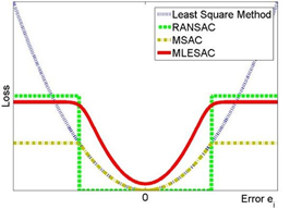
아래 사진은 몇몇 모델 근사 알고리즘의
loss error그래프로, RANSAC의 경우 에러가 임계값 이하일 때loss가 0인 것을 확인할 수 있다.
-
-
임계값
threshold민감성-
RANSAC은
threshold파라미터, 즉 임계값에 크게 영향을 받는다.
임계값을 너무 작게 설정하면 모델이 안정적으로fitting되지 않을 수 있고, 데이터의 변화에 너무 민감하게 반응할 수 있다. 또한 기준 이상의 모델을 찾는데 시간이 오래 걸릴 수 있다.
임계값을 너무 크게 설정하면outlier에 해당하는 값도inlier로 판단할 수 있어 바라는 최적의 모델을 찾을 수 없게 된다.
또한inlier의 분포가 변한다면 임계값 기준 또한 적응형adaptive으로 변해야 할 수 있다. -
이를 모두 고려하여 임계값
threshold을 정하는 것이 어렵다.
-
-
outlier가 특정 모델을 이루고 있을 경우-
만약
outlier가 노이즈 같지 않고 특정 구조, 분포를 이루고 있다면, 이러한outlier들이 샘플링되고 이에fitting한 잘못된 모델이 결과로서 출력될 수 있다. -
따라서 데이터셋을 미리 확인해
outlier가 특정 패턴 및 분포를 가지는 지 사전에 확인하고 제거해야 할 필요가 있다.
-
관련 항목
Lo-RANSAC
MLESAC
예시
의사코드와 이를 바탕으로 한 Python 코드
Given:
    data – A set of observations.
    model – A model to explain the observed data points.
    n – The minimum number of data points required to estimate the model parameters.
    k – The maximum number of iterations allowed in the algorithm.
    t – A threshold value to determine data points that are fit well by the model (inlier).
    d – The number of close data points (inliers) required to assert that the model fits well to the data.

Return:
    bestFit – The model parameters which may best fit the data (or null if no good model is found).


iterations = 0
bestFit = null
bestErr = something really large // This parameter is used to sharpen the model parameters to the best data fitting as iterations go on.

while iterations < k do
    maybeInliers := n randomly selected values from data
    maybeModel := model parameters fitted to maybeInliers
    confirmedInliers := empty set
    for every point in data do
        if point fits maybeModel with an error smaller than t then
             add point to confirmedInliers
        end if
    end for
    if the number of elements in confirmedInliers is > d then
        // This implies that we may have found a good model.
        // Now test how good it is.
        betterModel := model parameters fitted to all the points in confirmedInliers
        thisErr := a measure of how well betterModel fits these points
        if thisErr < bestErr then
            bestFit := betterModel
            bestErr := thisErr
        end if
    end if
    increment iterations
end while

return bestFitfrom copy import copy
import numpy as np
from numpy.random import default_rng
rng = default_rng()
class RANSAC:
def __init__(self, n=10, k=100, t=0.05, d=10, model=None, loss=None, metric=None):
self.n = n # `n`: Minimum number of data points to estimate parameters
self.k = k # `k`: Maximum iterations allowed
self.t = t # `t`: Threshold value to determine if points are fit well
self.d = d # `d`: Number of close data points required to assert model fits well
self.model = model # `model`: class implementing `fit` and `predict`
self.loss = loss # `loss`: function of `y_true` and `y_pred` that returns a vector
self.metric = metric # `metric`: function of `y_true` and `y_pred` and returns a float
self.best_fit = None
self.best_error = np.inf
def fit(self, X, y):
for _ in range(self.k):
ids = rng.permutation(X.shape[0])
maybe_inliers = ids[: self.n]
maybe_model = copy(self.model).fit(X[maybe_inliers], y[maybe_inliers])
thresholded = (
self.loss(y[ids][self.n :], maybe_model.predict(X[ids][self.n :]))
< self.t
)
inlier_ids = ids[self.n :][np.flatnonzero(thresholded).flatten()]
if inlier_ids.size > self.d:
inlier_points = np.hstack([maybe_inliers, inlier_ids])
better_model = copy(self.model).fit(X[inlier_points], y[inlier_points])
this_error = self.metric(
y[inlier_points], better_model.predict(X[inlier_points])
)
if this_error < self.best_error:
self.best_error = this_error
self.best_fit = better_model
return self
def predict(self, X):
return self.best_fit.predict(X)
def square_error_loss(y_true, y_pred):
return (y_true - y_pred) ** 2
def mean_square_error(y_true, y_pred):
return np.sum(square_error_loss(y_true, y_pred)) / y_true.shape[0]
class LinearRegressor:
def __init__(self):
self.params = None
def fit(self, X: np.ndarray, y: np.ndarray):
r, _ = X.shape
X = np.hstack([np.ones((r, 1)), X])
self.params = np.linalg.inv(X.T @ X) @ X.T @ y
return self
def predict(self, X: np.ndarray):
r, _ = X.shape
X = np.hstack([np.ones((r, 1)), X])
return X @ self.params
if __name__ == "__main__":
regressor = RANSAC(model=LinearRegressor(), loss=square_error_loss, metric=mean_square_error)
X = np.array([-0.848,-0.800,-0.704,-0.632,-0.488,-0.472,-0.368,-0.336,-0.280,-0.200,-0.00800,-0.0840,0.0240,0.100,0.124,0.148,0.232,0.236,0.324,0.356,0.368,0.440,0.512,0.548,0.660,0.640,0.712,0.752,0.776,0.880,0.920,0.944,-0.108,-0.168,-0.720,-0.784,-0.224,-0.604,-0.740,-0.0440,0.388,-0.0200,0.752,0.416,-0.0800,-0.348,0.988,0.776,0.680,0.880,-0.816,-0.424,-0.932,0.272,-0.556,-0.568,-0.600,-0.716,-0.796,-0.880,-0.972,-0.916,0.816,0.892,0.956,0.980,0.988,0.992,0.00400]).reshape(-1,1)
y = np.array([-0.917,-0.833,-0.801,-0.665,-0.605,-0.545,-0.509,-0.433,-0.397,-0.281,-0.205,-0.169,-0.0531,-0.0651,0.0349,0.0829,0.0589,0.175,0.179,0.191,0.259,0.287,0.359,0.395,0.483,0.539,0.543,0.603,0.667,0.679,0.751,0.803,-0.265,-0.341,0.111,-0.113,0.547,0.791,0.551,0.347,0.975,0.943,-0.249,-0.769,-0.625,-0.861,-0.749,-0.945,-0.493,0.163,-0.469,0.0669,0.891,0.623,-0.609,-0.677,-0.721,-0.745,-0.885,-0.897,-0.969,-0.949,0.707,0.783,0.859,0.979,0.811,0.891,-0.137]).reshape(-1,1)
regressor.fit(X, y)
import matplotlib.pyplot as plt
plt.style.use("seaborn-darkgrid")
fig, ax = plt.subplots(1, 1)
ax.set_box_aspect(1)
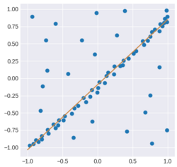
plt.scatter(X, y)
line = np.linspace(-1, 1, num=100).reshape(-1, 1)
plt.plot(line, regressor.predict(line), c="peru")
plt.show()- 결과
RANSAC, Lo-RANSAC - Python
RANSAC - Matlab
-
포물선 근사 문제를 RANSAC으로 풀어보도록 하자.
-
관측된 데이터 값들은 (x1, y1), ..., (xn, yn), 포물선의 방정식은 f(x) = ax2 + bx + c, 포물선을 결정하기 위해 뽑아야 할 샘플의 개수는 최소 3개이다.
-
c_max = 0 으로 초기화한다.
-
무작위로 세 점 p1, p2, p3를 뽑는다.
-
세 점을 지나는 포물선 f(x)를 구한다.
-
이렇게 구한 f(x)와의 거리 ri = |yi-f(xi)|가 T 이하인 데이터의 개수 c을 구한다.
-
만일 c가 c_max보다 크다면 현재 f(x)를 저장한다 (과거에 저장된 값은 버린다)
-
2~5 과정을 N번 반복한 후 최종 저장되어 있는 f(x)를 반환한다.
-
(선택사항) 최종 f(x)를 지지하는 데이터들에 대해 최소자승법을 적용하여 결과를 refine한다.
% input data

noise_sigma = 100;

x = [1:100]';

y = -2*(x-40).^2+30;

oy = 500*abs(x-60)-5000;

y([50:70]) = y([50:70]) + oy([50:70]);

y = y + noise_sigma*randn(length(x),1);


% build matrix

A = [x.^2 x ones(length(x),1)];

B = y;


% RANSAC fitting

n_data = length(x);

N = 100;        % iterations

T = 3*noise_sigma;   % residual threshold

n_sample = 3;

max_cnt = 0;

best_model = [0;0;0];

for itr=1:N,

    % random sampling

    k = floor(n_data*rand(n_sample,1))+1;


   % model estimation

    AA = [x(k).^2 x(k) ones(length(k),1)];

    BB = y(k);

    X = pinv(AA)*BB;  % AA*X = BB


   % evaluation

    residual = abs(B-A*X);

    cnt = length(find(residual<T));

    if(cnt>max_cnt),

        best_model = X;

        max_cnt = cnt;

    end;

end;


% optional LS(Least Square) fitting

residual = abs(A*best_model - B);

in_k = find(residual<T);    % inlier k

A2 = [x(in_k).^2 x(in_k) ones(length(in_k),1)];

B2 = y(in_k);

X = pinv(A2)*B2;    % refined model


% drawing

F = A*X;

figure; plot(x,y,'*b',x,F,'r');
활용 예
-
RANSAC (RANdom SAmple Consensus) 개념 및 실습 | Computer Vision에서의 RANSAC 활용
-
RANSAC - Random Sample Consensus | Cyrill Stachniss | RANSAC을 활용한 이미지 스티칭 등 활용 예시
참고
- Wikipedia | Random sample consensus
- RANSAC (RANdom SAmple Consensus) 개념 및 실습
- RANSAC의 이해와 영상처리 활용
- RANSAC - 5 Minutes with Cyrill
- RANSAC - Random Sample Consensus | Cyrill Stachniss
- 중학생도 이해할 수 있는 RANSAC 알고리즘 원리
- [시각지능] RANSAC
- Dealing with Outliers: RANSAC | Image Stitching
- Robust linear model estimation using RANSAC
- SLAM Online Study | SLAM DUNK Season 2 | RANSAC
- RANSAC (RANdom SAmple Consensus) Algorithm Implementation
- RANSAC Algorithm
- [Regressor] MLESAC
- New Approach for Regression Analysis – RANSAC and MLESAC