Maximum Likelihood Estimation Sample Consensus (MLESAC)

Introduction

The Maximum Likelihood Estimation SAmple Consensus (MLESAC) algorithm extends the Random Sample Consensus (RANSAC) methodology by incorporating a probabilistic framework for model fitting in data sets with significant outlier presence. When combined with an Ordinary Least Squares (OLS) model as the base estimator, MLESAC leverages the statistical properties of OLS to estimate parameters that maximize the likelihood, offering a robust approach to linear regression problems in noisy environments.

Background and Theory

MLESAC's integration with an OLS model represents a synthesis of probabilistic outlier handling and classical linear regression. The OLS model provides a simple, efficient way to estimate the parameters of a linear model by minimizing the sum of squared residuals. In the context of MLESAC, the OLS model is used to hypothesize the relationship within subsets of the data, while MLESAC evaluates these hypotheses through a probabilistic lens to determine the most likely model.

Mathematical Foundations

Consider a dataset $\{\mathbf{x}_i, y_i\}_{i=1}^N$, where $\mathbf{x}_i$ is a vector of explanatory variables and $y_i$ is the dependent variable for the $i$-th observation. The OLS model seeks to find the parameter vector $\boldsymbol{\beta}$ that minimizes the sum of squared residuals:

Under MLESAC, each hypothesis generated by fitting the OLS model to a randomly selected subset is assessed by computing the likelihood of the entire dataset given the model parameters. This likelihood is influenced by the assumption that inliers follow a Gaussian distribution around the regression line, while outliers are distributed uniformly.

Procedural Steps with OLS Base Estimator

1. Initialization: Specify the number of iterations, threshold for inlier classification, and criteria for model selection (e.g., maximum likelihood).
2. Hypothesis Generation and Evaluation:
   • For each iteration:
     • Randomly select a minimal subset of data points.
     • Fit an OLS model to this subset to estimate parameters $\boldsymbol{\beta}$.
     • Calculate the likelihood of each observation under this model, considering the Gaussian distribution for inliers and uniform distribution for outliers.
     • Determine the total likelihood of the dataset for this model.
3. Model Selection:
   • Identify the model with the highest total likelihood across all iterations.
   • Use all data points classified as inliers to refine the $\boldsymbol{\beta}$ estimate through a final OLS regression.

Mathematical Formulation

Maximizing the Likelihood Function

Given a dataset $\{\mathbf{x}_i, y_i\}_{i=1}^N$, where $\mathbf{x}_i$ is a vector of explanatory variables and $y_i$ is the dependent variable for the $i$-th observation, we assume that the errors $\epsilon_i = y_i - \mathbf{x}_i^T\boldsymbol{\beta}$ for inliers are normally distributed with mean 0 and variance $\sigma^2$. Thus, the probability density function (PDF) for the error of an inlier is given by:

The likelihood of observing a particular $y_i$ given $\mathbf{x}_i$ and $\boldsymbol{\beta}$ under this model is the same as the PDF of the error, since $y_i - \mathbf{x}_i^T\boldsymbol{\beta} = \epsilon_i$. Therefore, the likelihood function $L(\boldsymbol{\beta})$ for all observations is the product of the individual likelihoods:

To find the $\boldsymbol{\beta}$ that maximizes $L(\boldsymbol{\beta})$, it is common to maximize the log-likelihood (LL) because the logarithm is a monotonically increasing function that simplifies multiplication into addition, making the maximization problem more tractable:

The term $-\frac{1}{2}\log(2\pi\sigma^2)$ is constant with respect to $\boldsymbol{\beta}$, so maximizing LL with respect to $\boldsymbol{\beta}$ is equivalent to minimizing the sum of squared residuals $\sum_{i=1}^{N}(y_i - \mathbf{x}_i^T\boldsymbol{\beta})^2$, which is the objective function of OLS.

Derivation of $\boldsymbol{\beta}$

The OLS solution minimizes the sum of squared residuals:

This minimization problem leads to the normal equations:

where $\mathbf{X}$ is the matrix of explanatory variables (with each row corresponding to $\mathbf{x}_i^T$) and $\mathbf{y}$ is the vector of dependent variables $y_i$. The solution to these equations gives the estimate for $\boldsymbol{\beta}$:

This derivation illustrates that, within the MLESAC framework, when using an OLS base estimator, the process of fitting the model and evaluating hypotheses through likelihood maximization implicitly aligns with the OLS objective of minimizing the sum of squared residuals. This linkage between probabilistic model fitting and regression analysis not only underscores the robustness of combining MLESAC with OLS but also highlights the mathematical elegance of this approach in handling outliers in linear regression models.

Implementation

Parameters

• estimator: Estimator, default = LinearRegressor()
  Regression estimator
  
• min_points: int float, default = 2
  Mininum sample size for each random sample
  
• max_iter: int, default = 1000
  Maximum iteration
  
• min_inliers: int float, default = 0.5
  Minimum number of inliers for a model to be considered valid
  
• threshold: float, default = None
  Maximum distance a point can have to be considered an inlier
  
• random_state: int, default = None
  Seed for random sampling the data
  

Examples

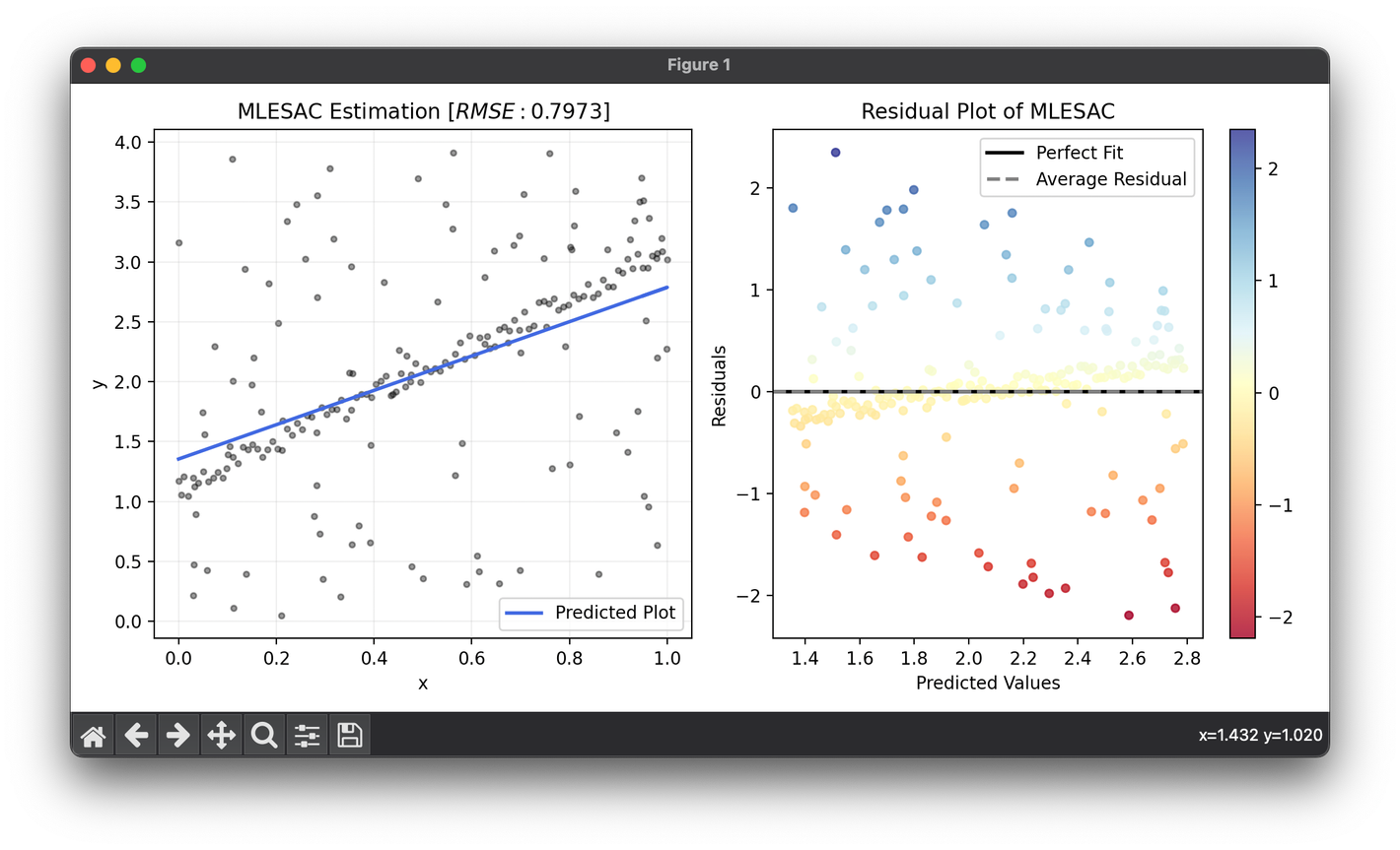
from luma.regressor.robust import MLESAC
from luma.metric.regression import RootMeanSquaredError
from luma.visual.evaluation import ResidualPlot

import matplotlib.pyplot as plt
import numpy as np

X = np.linspace(0, 1, 100)
y = 2 * X + 1 + 0.2 * np.random.rand(100)

noise = np.random.rand(100, 2)
X = np.vstack((X, noise[:, 0]))
y = np.hstack((y, 4 * noise[:, 1]))
X = X.reshape(-1, 1)

model = MLESAC(min_points=10, threshold=5)
model.fit(X, y)
score = model.score(X, y, metric=RootMeanSquaredError)

fig = plt.figure(figsize=(10, 5))
ax1 = fig.add_subplot(1, 2, 1)
ax2 = fig.add_subplot(1, 2, 2)

ax1.scatter(X, y, s=10, c="black", alpha=0.4)
ax1.plot(X, model.predict(X), lw=2, c="royalblue", label="Predicted Plot")
ax1.set_xlabel("x")
ax1.set_ylabel("y")
ax1.set_title(f"{type(model).__name__} Estimation [$RMSE:{score:.4f}$]")
ax1.legend()
ax1.grid(alpha=0.2)

res = ResidualPlot(model, X, y)
res.plot(ax=ax2, show=True)

Applications

• Computer Vision: For linear object detection and camera calibration.
• Econometrics: In robust regression analysis where data may be contaminated with outliers.
• Geosciences: For linear fitting in geological data analysis.

Strengths and Limitations

Strengths:

• Robustness: Offers robust parameter estimation in the presence of outliers.
• Statistical Basis: Combines the efficiency of OLS with a probabilistic model for outlier detection.

Limitations:

• Assumption of Linearity: Limited to linear models.
• Computational Cost: The iterative nature and likelihood calculations can be computationally intensive.

Advanced Topics

• Adaptive Thresholding: Dynamic adjustment of the inlier threshold based on data characteristics.
• Model Complexity: Extending the approach to handle polynomial and multi-dimensional OLS models.

References

1. Torr, P. H. S., and Zisserman, A. "MLESAC: A New Robust Estimator with Application to Estimating Image Geometry." Computer Vision and Image Understanding, vol. 78, no. 1, 2000, pp. 138-156.
2. Draper, N. R., and Smith, H. "Applied Regression Analysis." Wiley-Interscience, 1998.