🔎 Stanford CS231n 강의를 듣고 기록용도로 정리하는 게시글입니다.
Unsupervised Learning
Supervised Learning
- Data: (
x,y) wherexis data,yis label - Goal: Learn a function to map x → y
- Examples: Classification, regression, object detection, semantic segmentation, image captioning, etc.
Unsupervised Learning
- Data:
x(Just data, no labels!)- training data is cheap
- Goal: Learn some underlying hidden structure of the data
- Examples: Clustering, dimensionality reduction, feature learning, density estimation, etc.
Generative Models
- Given training data, generate new samples from same distribution
- class of models for unsupervised learning
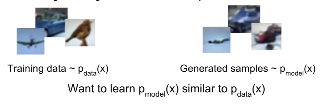
- class of models for unsupervised learning
- Addresses(다루다) density estimation, a core problem in unsupervised learning
- Explicit density estimation: explicitly define and solve
- Implicit density estimation: learn model that can sample from without explicitly defining it
- Why Generative models?
- realistic samples for artwork, super-resolution, colorization, etc.
- Generative models of time-series data can be used for simulation and planning (reinforcement learning applications)
- can also enable inference of latent representations that can be useful as general features
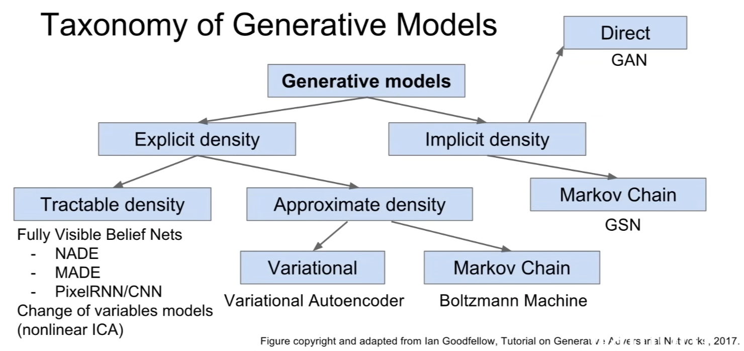
- Taxonomy(분류 체계) of Generative Models
PixelRNN and PixelCNN
- Fully visible belief network
- Explicit density model
- Use chain rule to decompose likelihood of an image
xinto product of 1-d distributions:
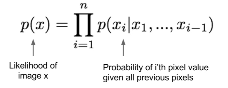
- image data
x, we want to model the probability of this imageP(x)
- image data
- Training the model - maximize the likelihood of training data
- However, the distribution of pixel values ( of given all the previous s) → very complex distribution
- how to mild this? → Express using a neural network
- but how do we order the pixels? what does 'all previous pixels' mean?
- how to mild this? → Express using a neural network
PixelRNN
- 2016
- defines a way for setting up and optimizing the problem
- generate image pixels starting from corner
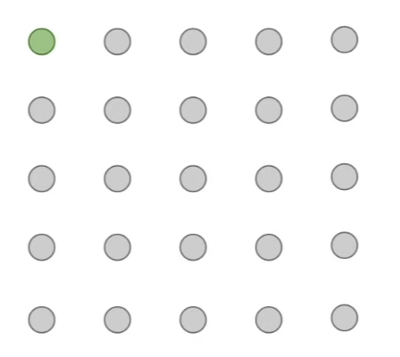
- then sequentially generate pixels based on the connections from the arrows
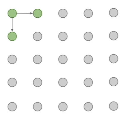
- dependency on previous pixels modeled using an RNN (LSTM)
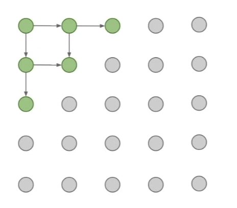
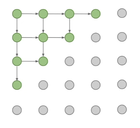
- continue moving down along the diagonal and generating all of these pixel values dependent on the pixels that they're connected to
- Drawback: sequential generation is slow
PixelCNN
- 2016
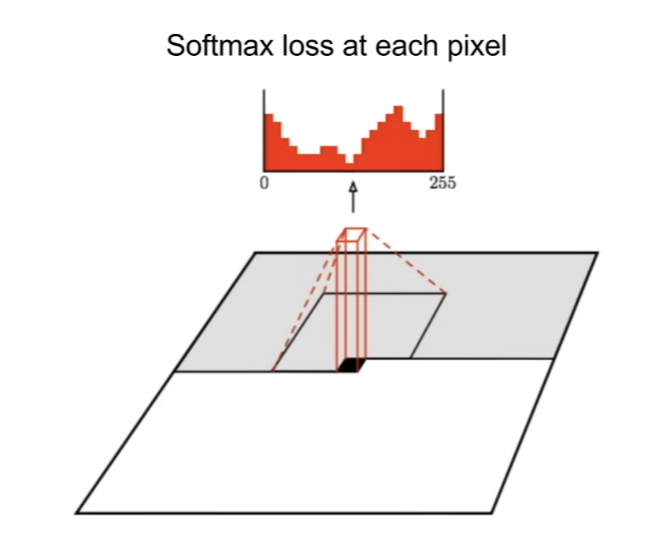
- Still generate image pixels starting from corner (and expanding outwards)
- Dependency on previous pixels now modeled using a CNN over context region
- this is a CNN at each pixel location → output of this = softmax loss over the pixel values
- training: by maximizing likelihood of training images
- at each pixel location, we have the ground truth training data image, which is basically the classification label that we want our pixel to be which of these 255 values, and train this using a softmax loss
Q: Why do we have a classification label here when it's unsupervised learning?
A: This loss, the output that we have is the value of the input training data. So, we have no external labels. Just taking the input data and saying that this is what we used for the loss function.
- We're outputting a distribution over pixel values at each location of the image, and what we want to do is to maximize the likelihood of input(=training data) being produced (=generated) → use input to create the loss
- Training is faster than PixelRNN
- can parallelize convolutions since context region values known from training images
- Generation must still proceed sequentially
- still slow
- at test time where we generate a completely new image, we have to generate each of the pixel locations before we can generate the next location
PixelRNN and PixelCNN
- Pros
- Can explicitly compute likelihood p(x)
- Explicit likelihood of training data gives good evaluation metric
- Good samples
- Cons
- Sequential generation ⇒ slow
- Improving PixelCNN performance
- Gated convolutional layers
- Short-cut connections
- Discretized logistic loss
- Multi-scale
- Training tricks
- Etc...
- See
- Van der Oord et al. NIPS 2016
- Salimans et al. 2017 (PixelCNN+)
Variational Autoencoders (VAE)
- define intractable density function with latent :
- cannot optimize directly, derive and optimize lower bound on likelihood instead
Background: Autoencoders
- not to generate data, but an unsupervised approach for learning a lower dimensional feature representation from unlabeled training data
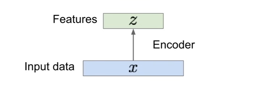
- have input data , and want to learn features,
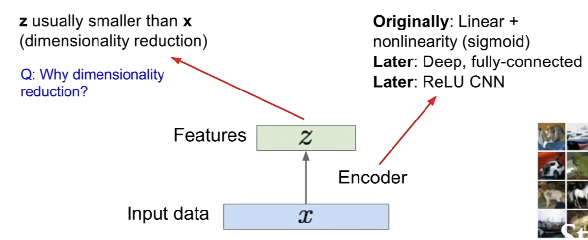
- have an encoder which is a function mapping from this input data to feature
- is usually smaller than , so we do dimensionality reduction
- Q: Why do we do dimensionality reduction? Why do we want to be smaller than ?
- We want to be able to learn features that can capture meaningful factors of variation in the data
Learning feature representation
- how to learn this feature representation?
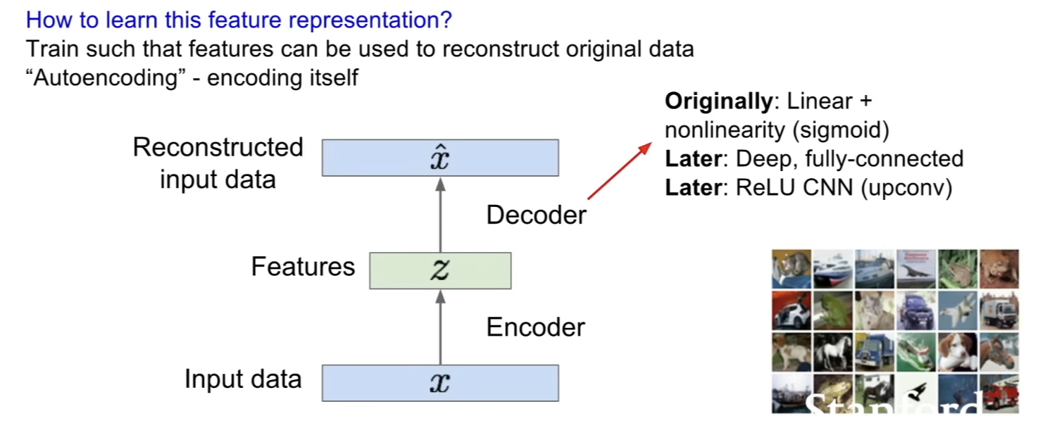
- take the features that were produced based on the output of the encoder, and use the decoder (second network) to output something of the same size dimensionality to and of similar to
- for the decoder, using same types of networks as encoders
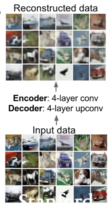
- reason why we have a conv network for encoder and upconv network for decoder
- at the encoder, we take the high dimensional input to lower dimensional features
- at the decoder, we want to go the other way (go from low dimensional features back out to high dimensional reconstructed input)
Loss function
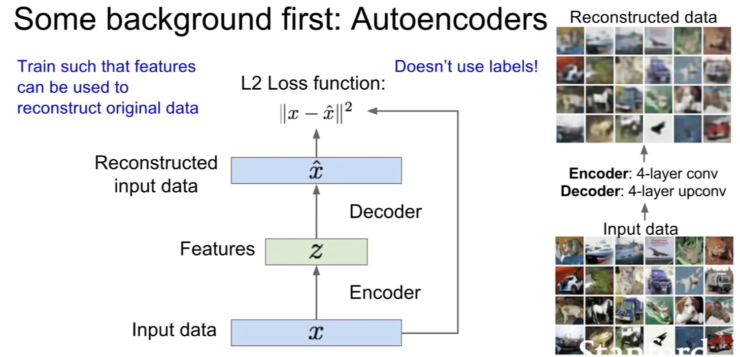
- using L2 loss functions; make the pixels of the reconstructed data to be the same as the input data
- even though we have loss function, there's no external labels that are being used in training this
- all we have is the training data that we're going to use to pass through the network as well as to compute the loss function
After training
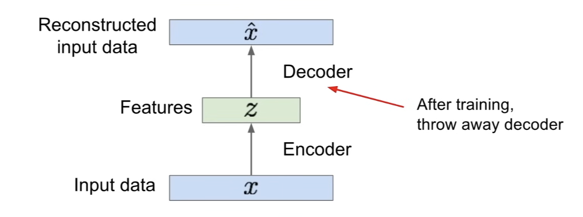
- after training this model, we can throw away the decoder
- purpose of the decoder was to produce reconstruction input and to compute loss function
-
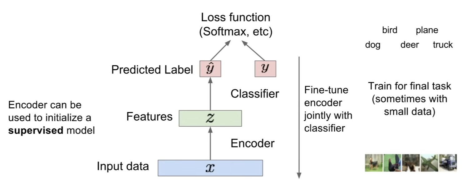
use the encoder that produces our feature mapping to initialize supervised model
-
now we can go from the input data to the features and then have an additional classifier network on top of this so that now we can use to output a class label
-
value: we were able to use a lot of unlabeled training data to try and learn good general feature representations
- now we can use this to initialize a supervised learning problem where sometimes there's not much data (only small data)
- allows you to initialize the model with better features
Variational Autoencoders
-
in Autoencoders, features capture factors of variation in training data
- now, can we generate new images from an autoencoder?
-
Probabilistic spin on autoencoders - will let us sample from the model to generate data
-
Assume training data is generated from underlying unobserved (latent) representation
- so, is a vector where each element is capturing how little or much of some factor of variation we have in the training data
- ex) when generating faces; how much of a smile is on the face, position of the eyebrows, orientation of the head
- so, is a vector where each element is capturing how little or much of some factor of variation we have in the training data
-
In generation process, sample from a prior over
- for each of the attributes (ex. how much smile there is), we can have a prior over what sort of distribution we think that there should be for this
- ex) a Gaussian is something that's a natural prior that we can use for each of the factors of
- then, generate data by sampling from a conditional distribution
- for each of the attributes (ex. how much smile there is), we can have a prior over what sort of distribution we think that there should be for this
-
so, we're sampling , sample a value for each of the latent factors, then use that to sample the image from here
-
true parameter of the generation process:
- parameters of the prior and conditional distributions
-
in order to have a generative model that can generate new data, we estimate the true parameters
How should we represent this model?
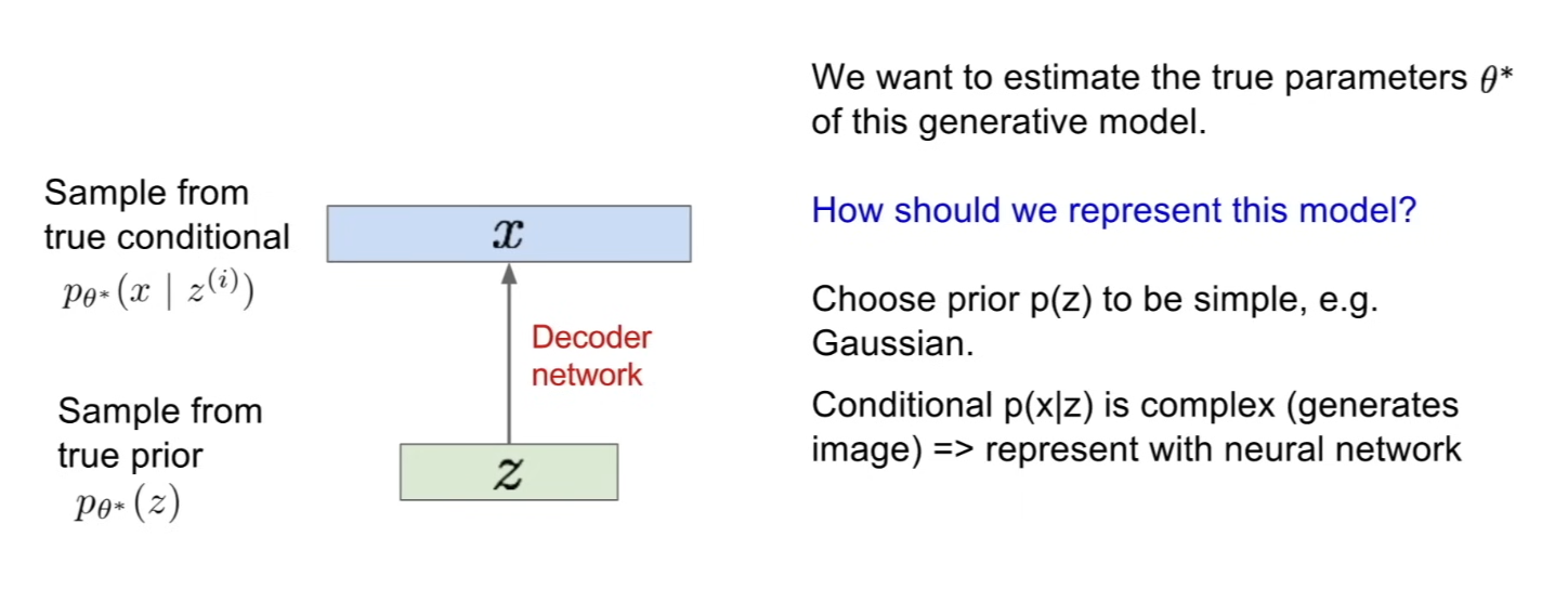
- for a model for this generator, we can choose prior to be simple, something like Gaussian
- reasonable choice for latent attributes
- now, is much more complex, b/c we need to use this to generate an image
- but when we have some type of complex function that we want to represent, we can represent this with neural network
- so, try with a neural network
How to train the model?
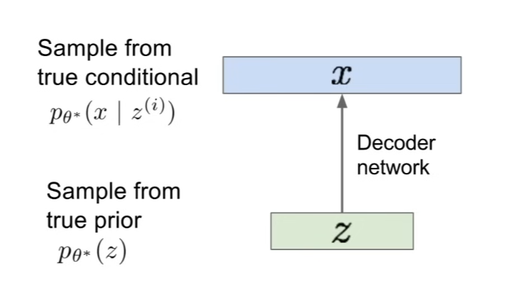
-
now calling network a decoder network
- taking some latent representation and trying to decode this into the image that it's specifying
- we want to train this model to learn an estimate of these parameters
-
remember strategy from training generative models, back from fully visible belief networks, PixelRNN, PixelCNN ⇒ a straightforward natural strategy is to try and learn these model parameters in order to maximize the likelihood of the training data
- in this case, with latent variable , we'll have to write out taking expectation over all possible values of , which is continuous
- but the problem here is that this integeral is not going to be tractable(다루기 쉬운)
Intractability
- Data likelihood:
- 1st term, - like mentioned above, we can choose this to be a simple Gaussian prior ⇒ fine
- 2nd term, - we said we're going to specify a decoder neural network, so given any , we can get from here (= output of the neural network) ⇒ fine
- integral - if we want to compute for every , we can't compute this integral (=intractable)
- Posterior density is also intractable: (by Bayes' rule)
- b/c is intractable data likelihood
- Solution: In addition to decoder network that models , define an additional encoder network that approximates
- calling this "encoder" because we want to get the likelihood of , so encode input data into
- this allows us to derive a lower bound on the data likelihood that is tractable, which we can optimize
Back to training
- in VAE, we want to model probabilistic generation of data
- like Autoencoder, we have an encoder and decoder but make them probabilistic
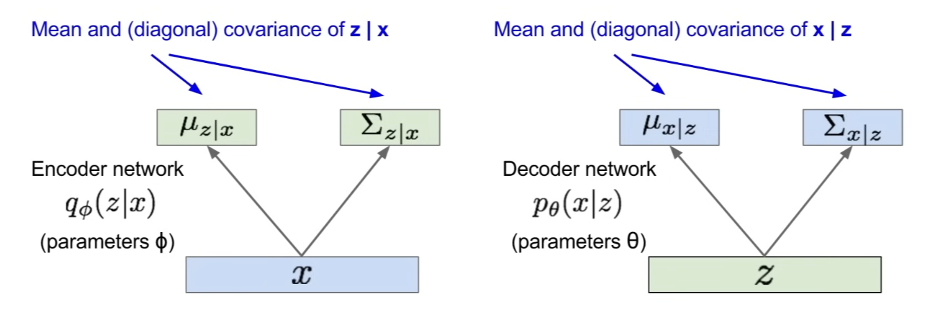
- encoder network, (parameter: ) - output a mean and a diagonal covariance
- 공분산: 두 확률변수 X, Y가 있을 때, 둘 사이에 상관관계가 존재하는지를 살펴보기 위해 공분산 사용함
- 공분산 > 0 = 양의 상관관계 / 공분산 = 0 = 둘이 상관관계 없음 / 공분산 < 0 = 음의 상관관계
- x의 편차와 y의 편차를 곱한 값의 평균
- 공분산: 두 확률변수 X, Y가 있을 때, 둘 사이에 상관관계가 존재하는지를 살펴보기 위해 공분산 사용함
- decoder network, (parameter: ) - starting from , output the mean and the diagonal covariacne of some ( is same dimension as the input )
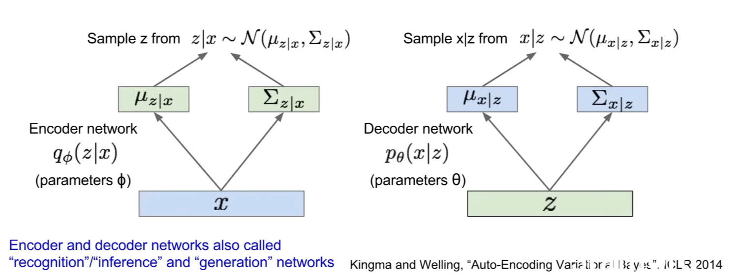
- now, in order to get our and , sample from the distributions
- encoder and decoder network are producing distributions over and , so we'll sample from this distribution in order to get a value from here
- encoder network is called "recognition/inference" network
- b/c we're trying to form inference of this latent representation of
- decoder network is called "generation" network
- b/c we'll use this to perform generation
Likelihood lower bound equation
- Now equipped with our encoder and decoder networks, work out the log (data likelihood)
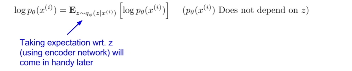
- 샘플링한 에 대한 의 기대값
- 의 분포에서 샘플링한 값인
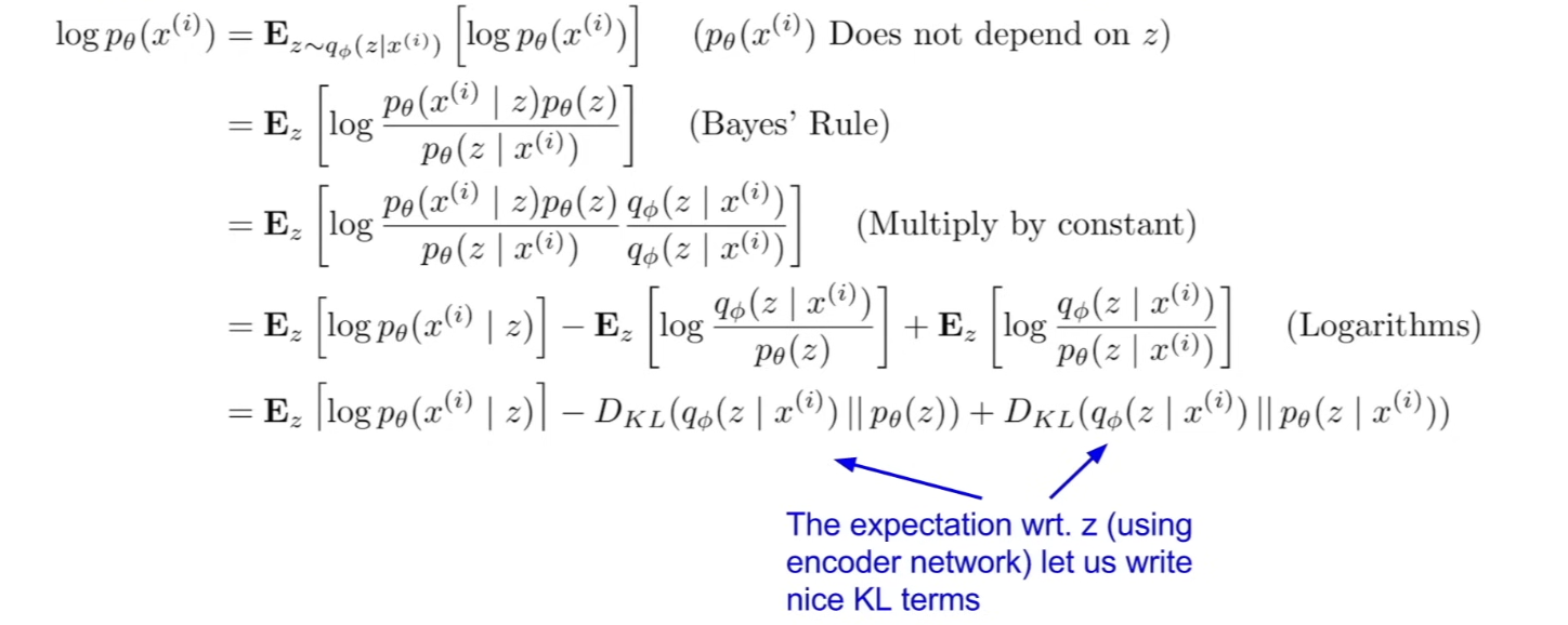
- 마지막 수식의 첫번째 항: 의 기댓값
- 마지막 수식의 나머지 두 항: KL diveregence항 (두 확률 분포의 차이를 구할 때 사용하는 함수, how close these 2 distributions are)
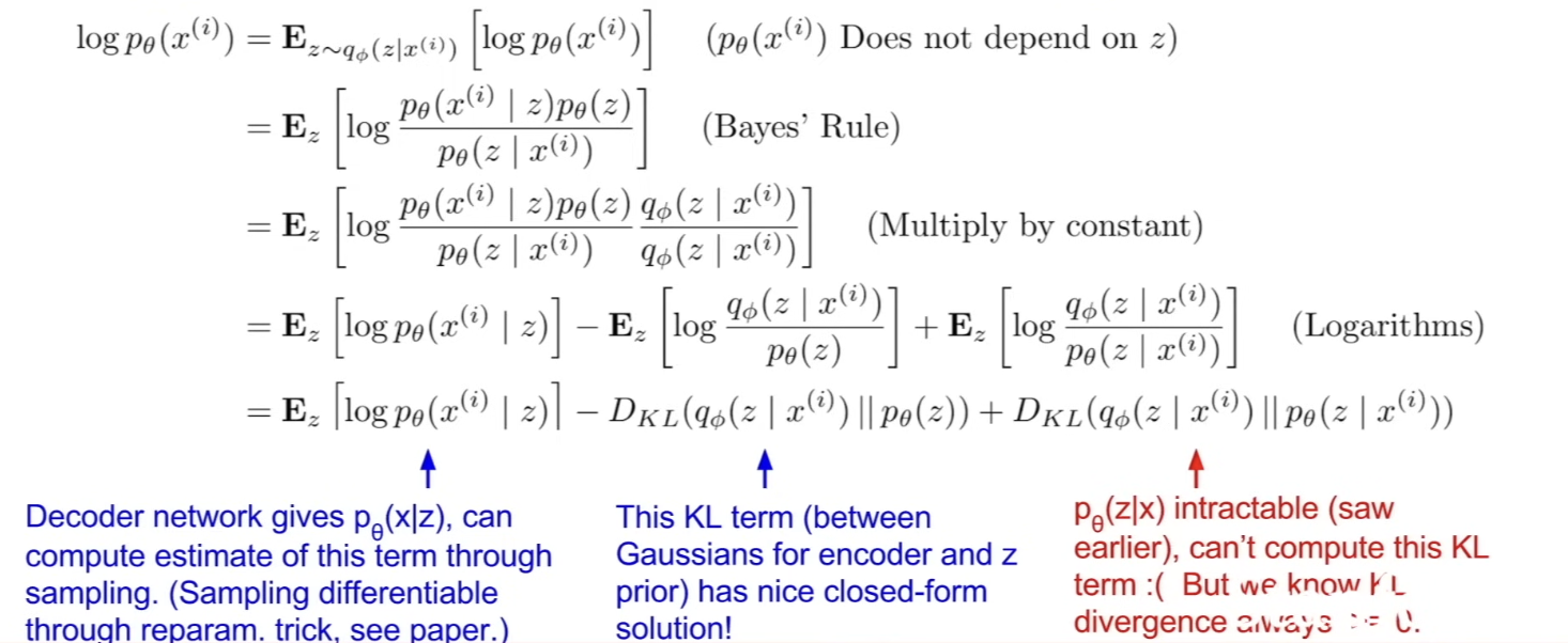
- first term = - provided by our decoder network. we're able to compute the estimate of this term through sampling. we can do a sampling that's differentiable(미분가능한) through something called re-parameterization trick
- second term = - a KL term between 2 Gaussians
- third term = - is intractable, that's why we used the estimate using ⇒ this term is a problem (But we know that KL divergence is >= 0)
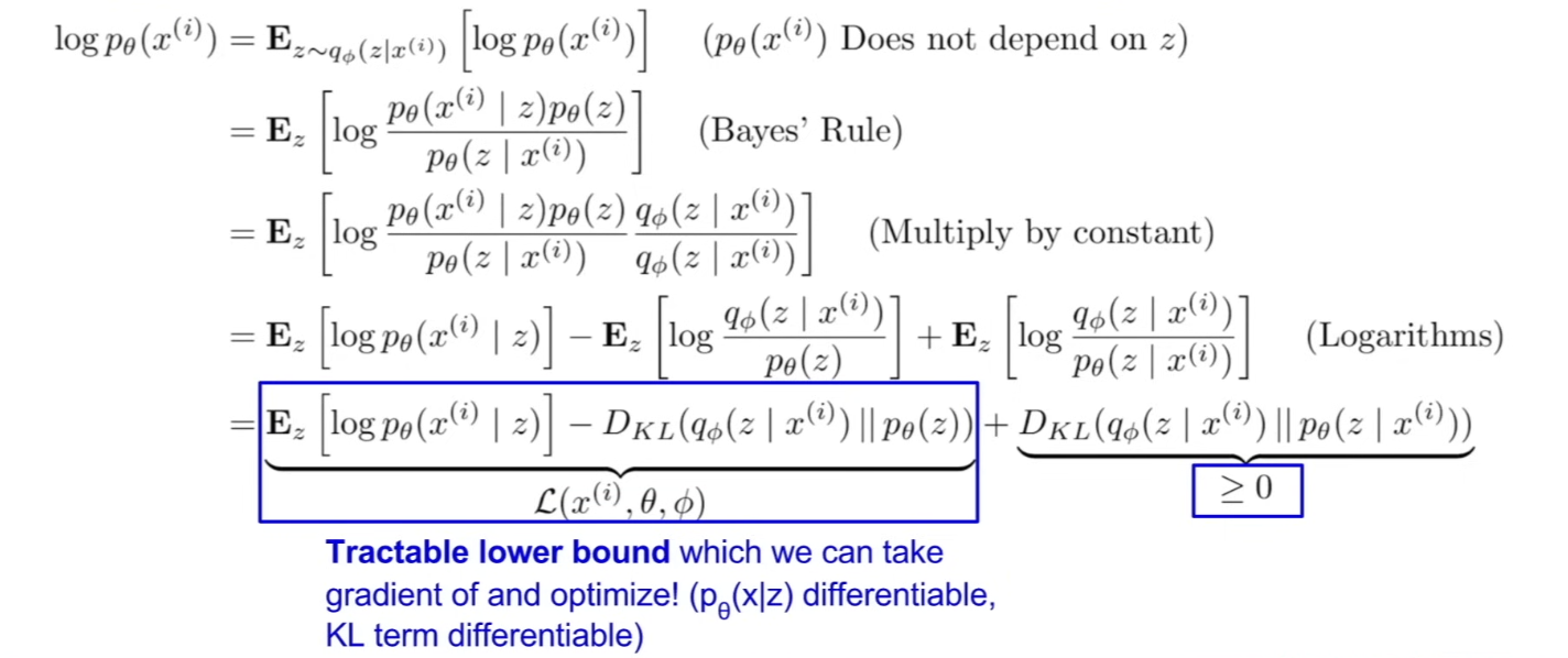
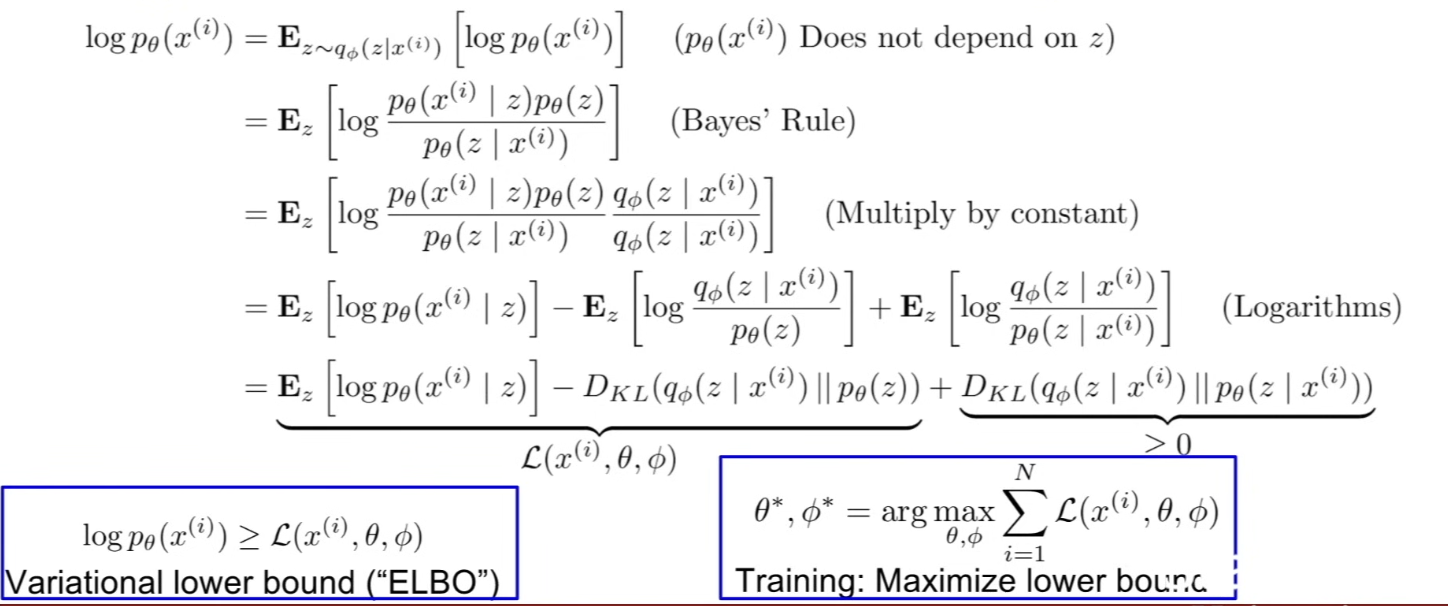
- so, we optimize and maximize the lower bound ⇒ we want to find the parameters that allows us to maximize this
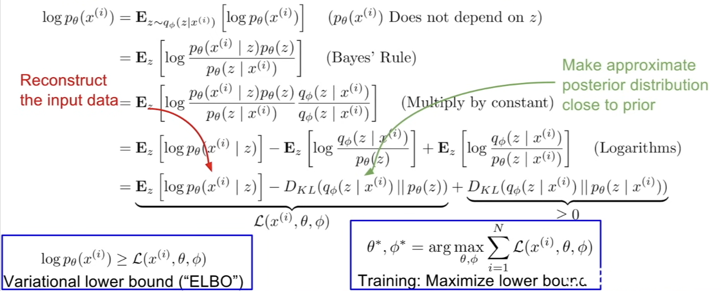
- first term - 기댓값이 크려면 결국 안의 확률 값이 커야 함 → reconstructing the data = similar to autoencoder
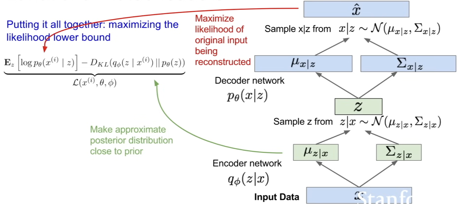
- second term - 이 KL 항을 작게 만들어야 함. which means to make approximate posterior distribution close to prior distribution = latent variable to have this distribution type(shape)
Maximizing the likelihood lower bound
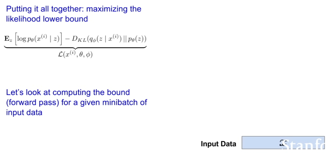
- when doing forward pass, we have input data (=mini-batch of the input data)
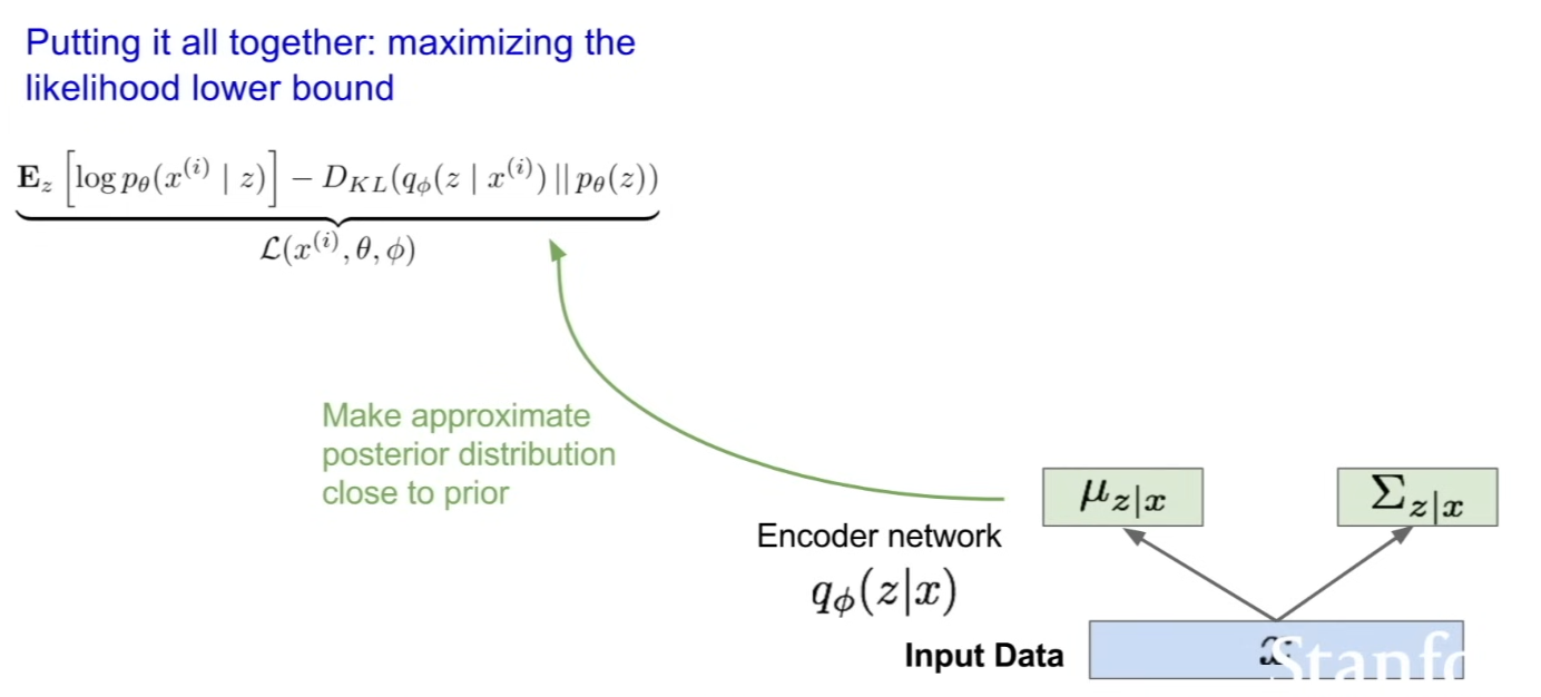
- pass it through encoder network → get
- then, from this , this is the term that we use to compute the KL term
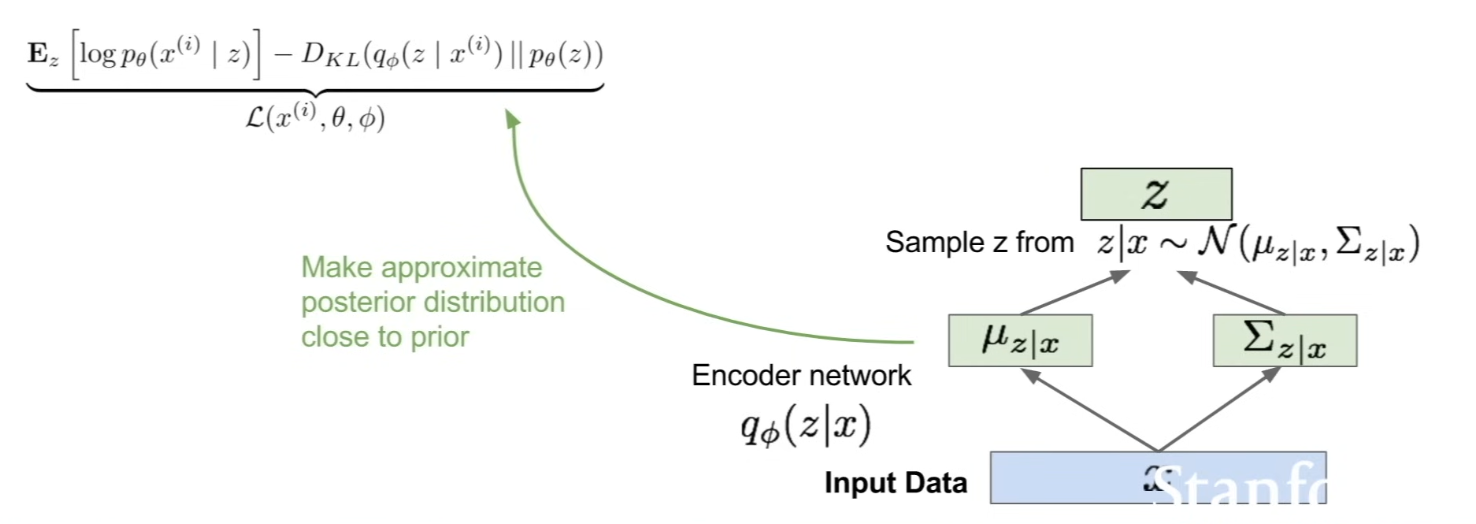
- sample from the distribution of ⇒ so we have a sample of the latent factors that we can infer from
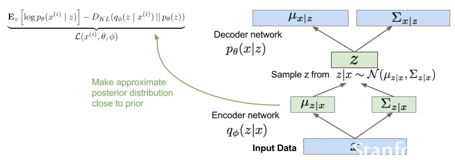
- then, pass the through the decoder network, and get the output of the mean and variance of the distribution
-
finally sample from this distribution and this will produce some sample output
-
when training, we'll take this distribution and say the loss term will be
-
so, we're maximizing the likelihood of this original input being reconstructed
-
now, for every mini-batch of the input, compute this forward pass and then backprop
Generating Data
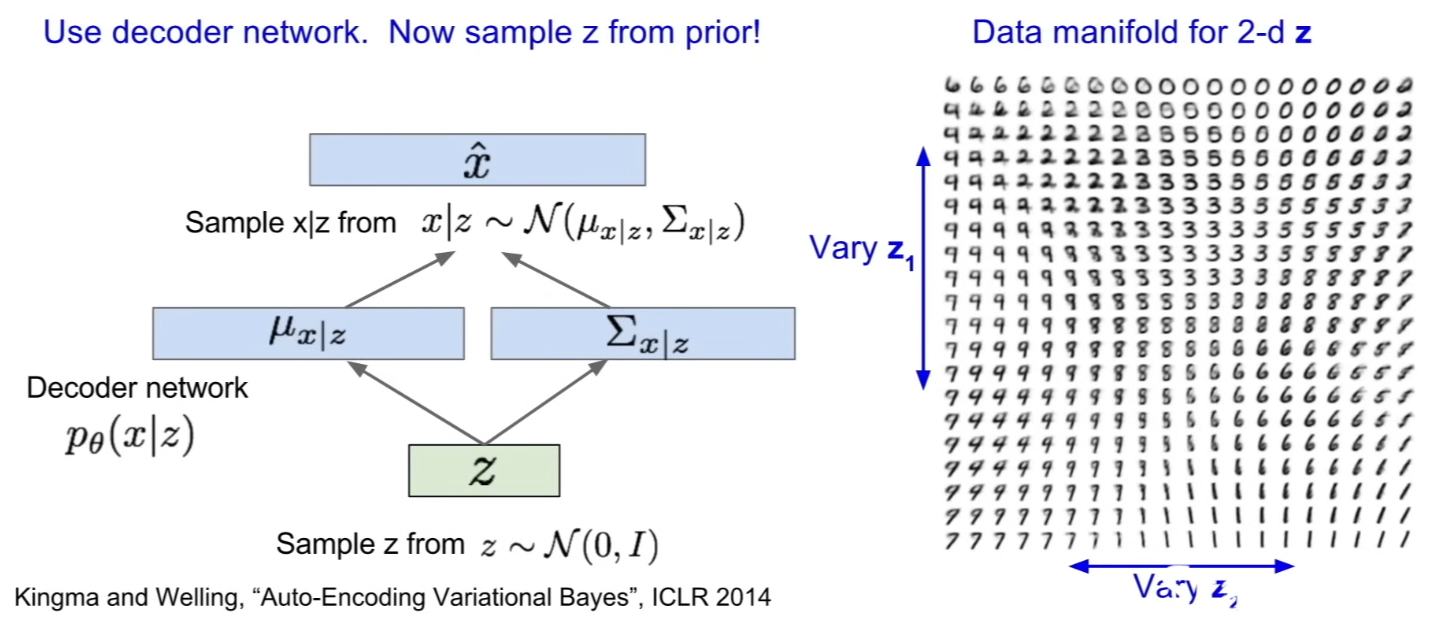
- after training, when we want to generate the data, we can use just the decoder network
- now, we can sample from the true generative process, instead of sampling from the posterior that we had during training
- which means that we sample from the prior that we specify
- then, sample our data from here
- if we have a 2D , and we take from the range of different percentiles of the distribution, and we vary and
- you can see that the image generated from every combination of and that we have here, is transitioning smoothly across all of the different variations
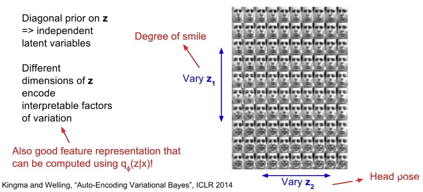
- we have chosen the prior on to be diagonal in order to encourage this to be independent latent variables that can then encode interpretable factors of variation
- b/c of this, we'll have different dimensions of , encoding different interpretable factors of variation
- in the example trained on faces, as we vary , going up and down, the amount of smile is changing
- as we vary , from left to right, the head pose is changing
Summary
- Probabilistic spin to traditional autoencoders ⇒ allows generating data
- Defines an intractable density ⇒ derive and optimize a (variational) lower bound
- Pros:
- Principled approach to generative models
- Allows inference of , can be useful feature representation for other tasks
- Cons:
- Maximizes lower bound of likelihood: okay, but not as good evaluation as PixelRNN/PixelCNN
- Samples blurrier and lower quality compared to state-of-the-art (GANs)
- Active areas of research:
- More flexible approximations, e.g. richer approximate posterior instead of diagonal Gaussian
- Incorporating structure in latent variables
Generative Adversarial Networks (GAN)
-
So far, PixelCNNs define tractable density function and optimize likelihood of training data / VAEs define intractable density function with latent , but cannot optimize directly, so derive and optimize lower bound on likelihood instead
-
What if we give up on explicitly modeling density, and just want the ability to sample?
⇒ GANs: don't work with any explicit density function. instead, take game-theoretic approach: learn to generate from training distribution through 2-player game -
Problem: Want to sample from complex, high-dimensional training distribution. But no direct way to do this
-
Solution: Sample from a simpler distribution, e.g. random noise. Learn transformation to training distribution.
-
Q: What can we use to represent this complex transformation?
- A neural network
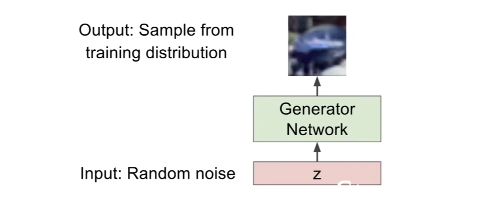
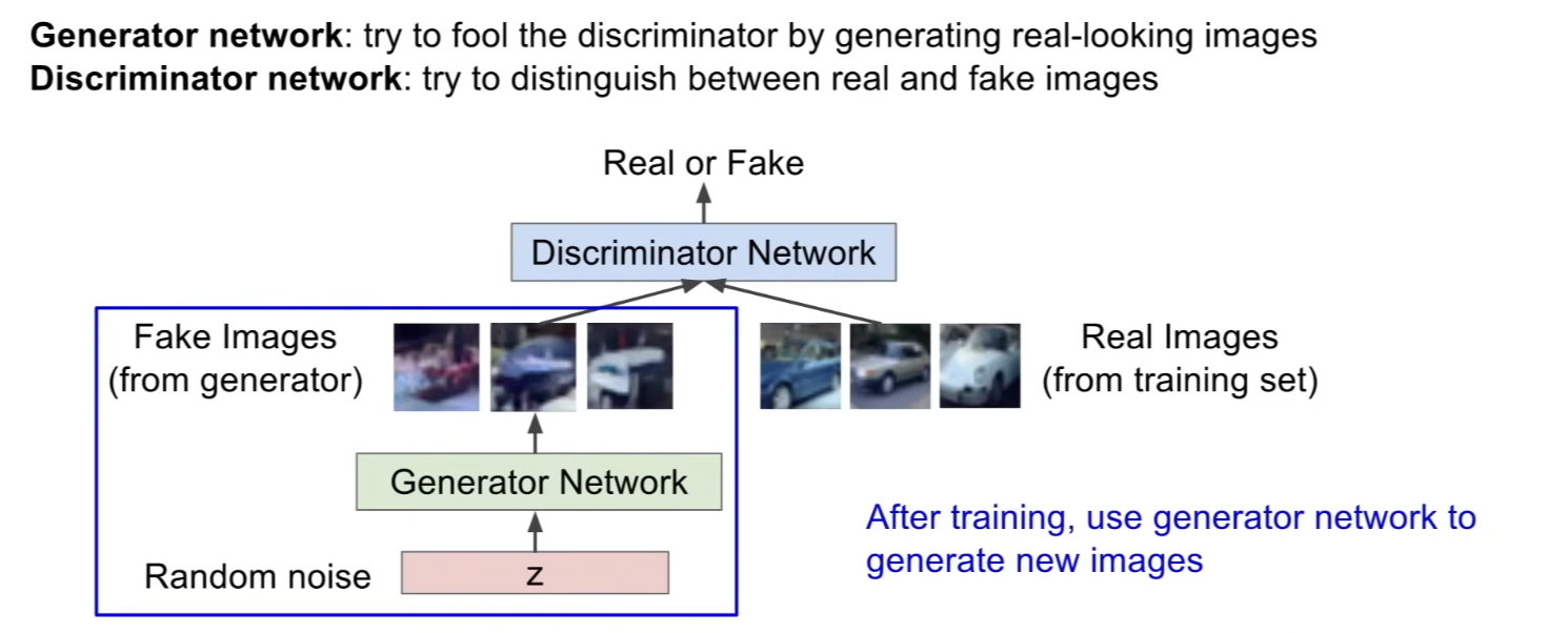
- in the GAN setup, take an input which is a vector of some dimension that we specify of random noise, and pass this through a generator network, then get as output a direct sample from the training distribution
- every input of random noise → corresponds it to a sample from the training distribution
Training GANs: Two-player game
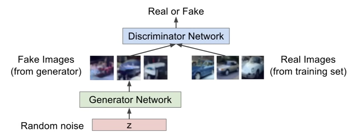
- Generator network: try to fool the discriminator by generating real-looking images
- Discriminator network: try to distinguish between real and fake images
- idea is that if the discriminator can do a good job of discriminating real vs. fake, and if the generator can generate fake images that can successfully fool the discriminator ⇒ we have a good generative model
- train jointly in minimax game

- : parameter of generator network G
- : parameter of discriminator network D
- 1st term: expectation over data of
- is the discriminator output for real data
- likelihood of real data being real from the data distribution
- 2nd term: expectation of drawn from (= samples from the generator network)
- = output of the discriminator for generated fake data ( = fake data))
- Discriminator() wants to maximize objective such that is close to 1(=real) and is close to 0(=fake)
- Generator() wants to minimize objectivesuch that is close to 1 (= discriminator is fooled into thinking generated is real)
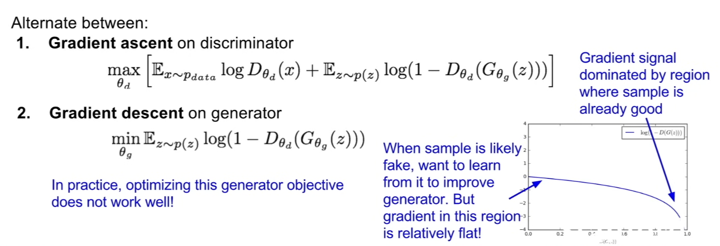
1. Gradient ascent on discriminator - learn that's maximizing this objective
2. Gradient descent on generator - only take the right part b/c that's the only part that's dependent on parameter
- in practice, the generator objective actually doesn't work well
- look at the loss landscape (x축: )
- if we apply (=what we want to minimize for the generator), it turns out the slope of this loss is going to be higher towards the right (=higher when is closer to 1)
- this means that when the generator is doing a good job of fooling the discriminator, we'll have a high gradient
- on the other hand, when we have bad samples (=generator has not learned a good job yet), then the discriminator can easily tell → now closer to the 0 region on the x axis → gradient is relatively flat
- this means that gradient signal is dominated by region where the sample is already pretty good, whereas we actually want to learn a lot when the samples are bad
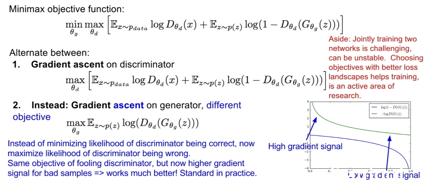
- in order to improve learning, define a different objective function for the gradient, where now we'll do gradient ascent instead
- instead of minimizing the likelihood of discriminator being correct(=what we did earlier),
- maximize the likelihood of discriminator being wrong
- now, we have a high gradient signal region on the left where we have bad samples, and now the flatter region is to the right where we have good samples
- it's hard to learn 2 networks at once, and there's issue of depending on what the loss landscape looks at, it can affect training dynamics
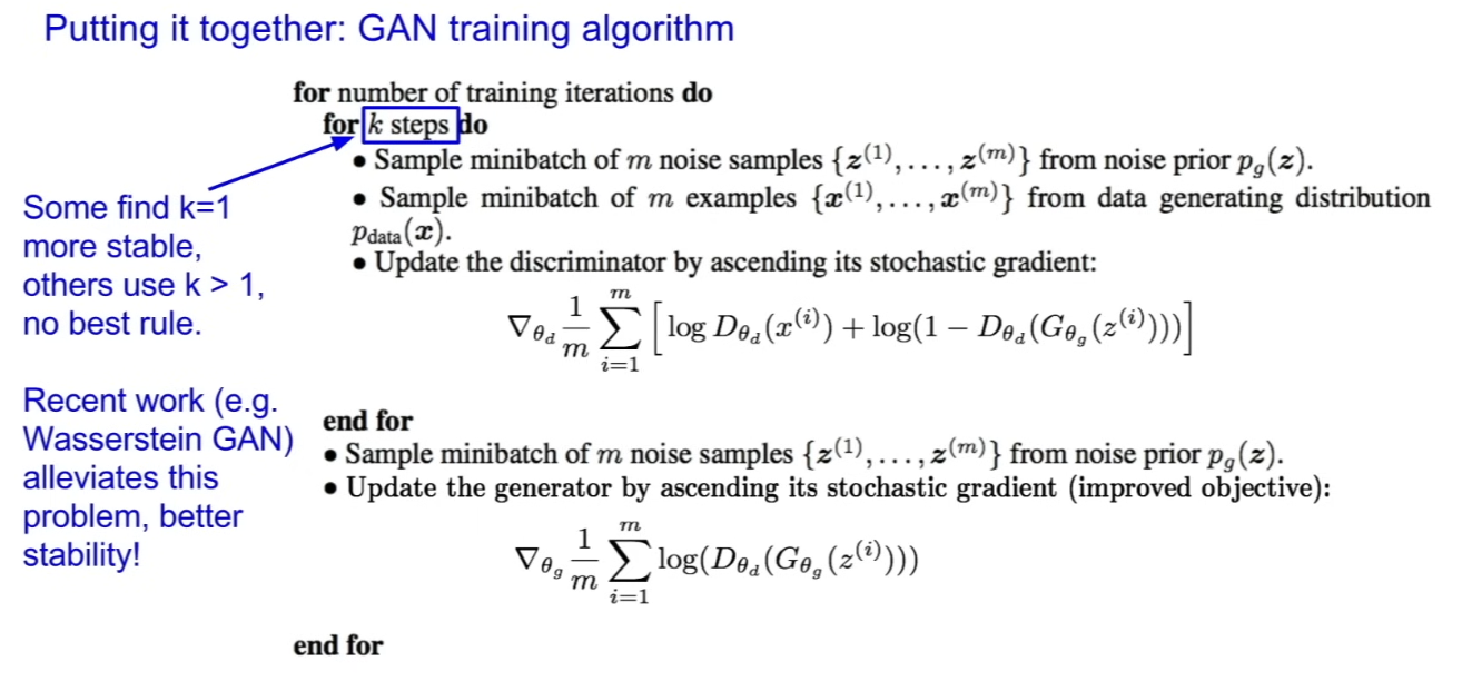
- for each iteration of training, train the discriminator and then generator
- for steps of training the discriminator network,
a. sample a minibatch noise samples from noise prior
b. sample a minibatch samples of real samples from training data
c. pass the noise through the generator → get fake images as output
d. take a gradient step on discriminator using this mini batch(fake and real images)
e. update discriminator parameters - sample a mini batch of noise samples
- pass this through the generator
- backprop on this to optimize the generator objective (have the generator fool the discriminator as much as possible)
- there's no clear rule to choose the value of for things to work better
Examples
GAN: Convolutional Architectures
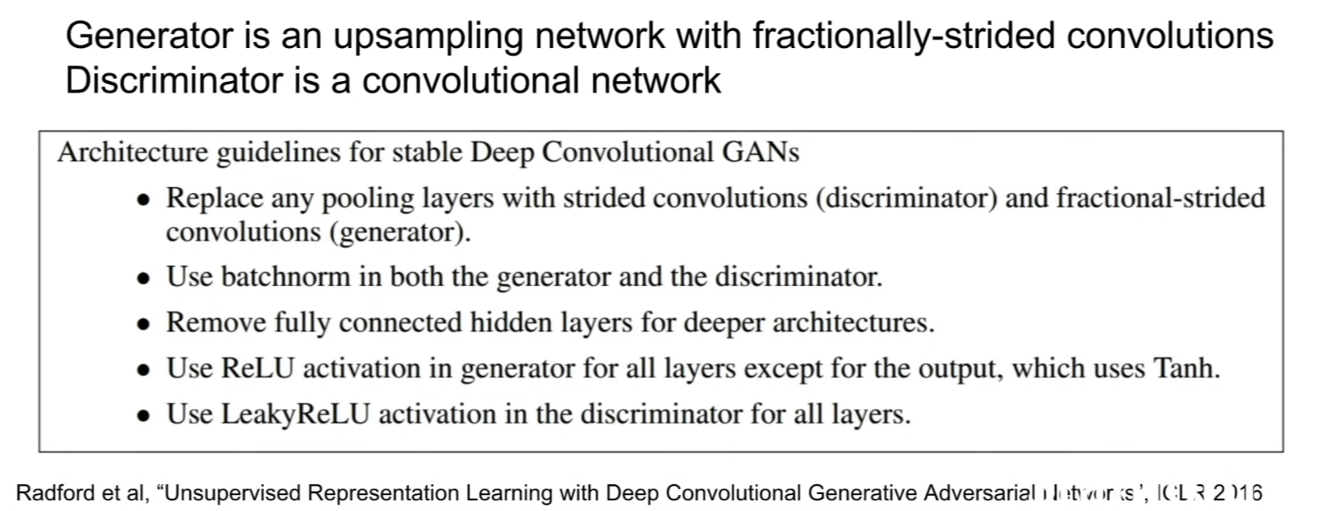
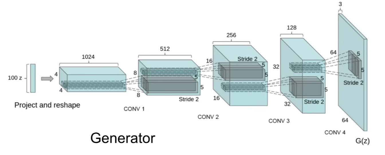
- going from input (=noise vector) and transforming this all the way to the output sample
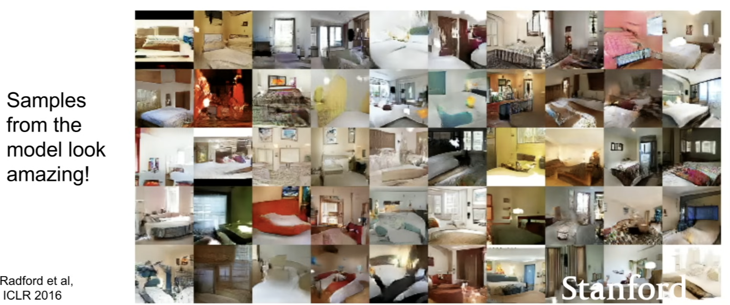
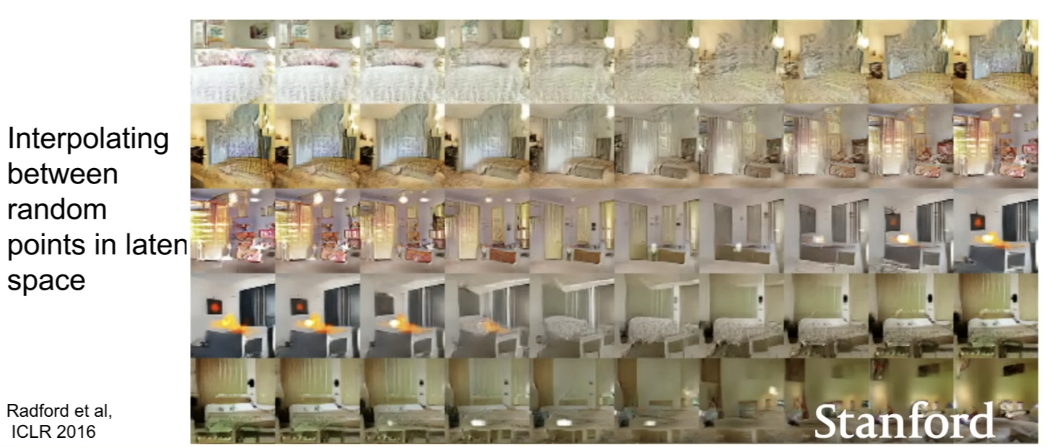
- interpreting what these GANs are doing
- take 2 points of , and interpolate between these points
- each row is an interpolation from one random noise to another random noise vector
- as it's changing, it's smoothly interpolating the image all the way over
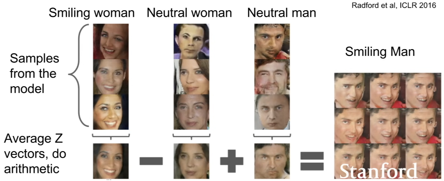
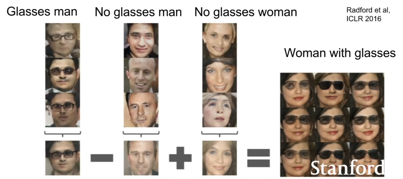
GAN: Interpretable Vector Math
-
analyzing what the vectors mean
-
here, it's sampling smiling woman, neutral woman, and neutral man
-
and, take the average of vectors that produced each of the samples
-
take the mean vector for smiling woman and subtract it by the mean vector for the neutral woman, and add the mean vector for neutral man ⇒ we get smiling man
GAN zoo
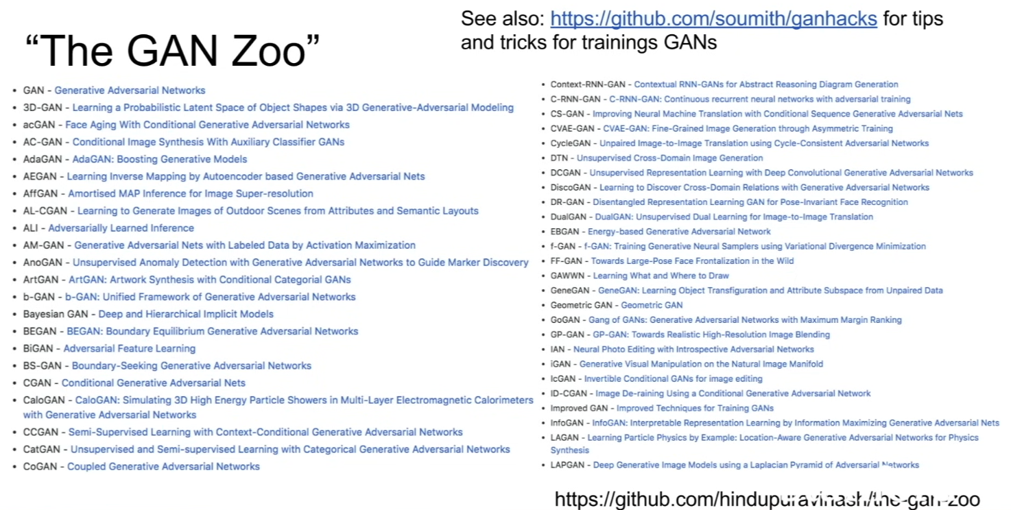
- See also: https://github.com/soumith/ganhacks for tips and tricks for training GANs
Summary
- Don't work with an explicit density function
- Take game-theoretic approach: learn to generate from training distribution through 2-player game
- Pros:
- Beautiful, state-of-the-art samples
- Cons:
- Trickier / more unstable to train
- Can't solve inference queries such as p(x), p(z|x)
- Active areas of research:
- Better loss functions, more stable training (Wasserstein GAN, LSGAN, many others)
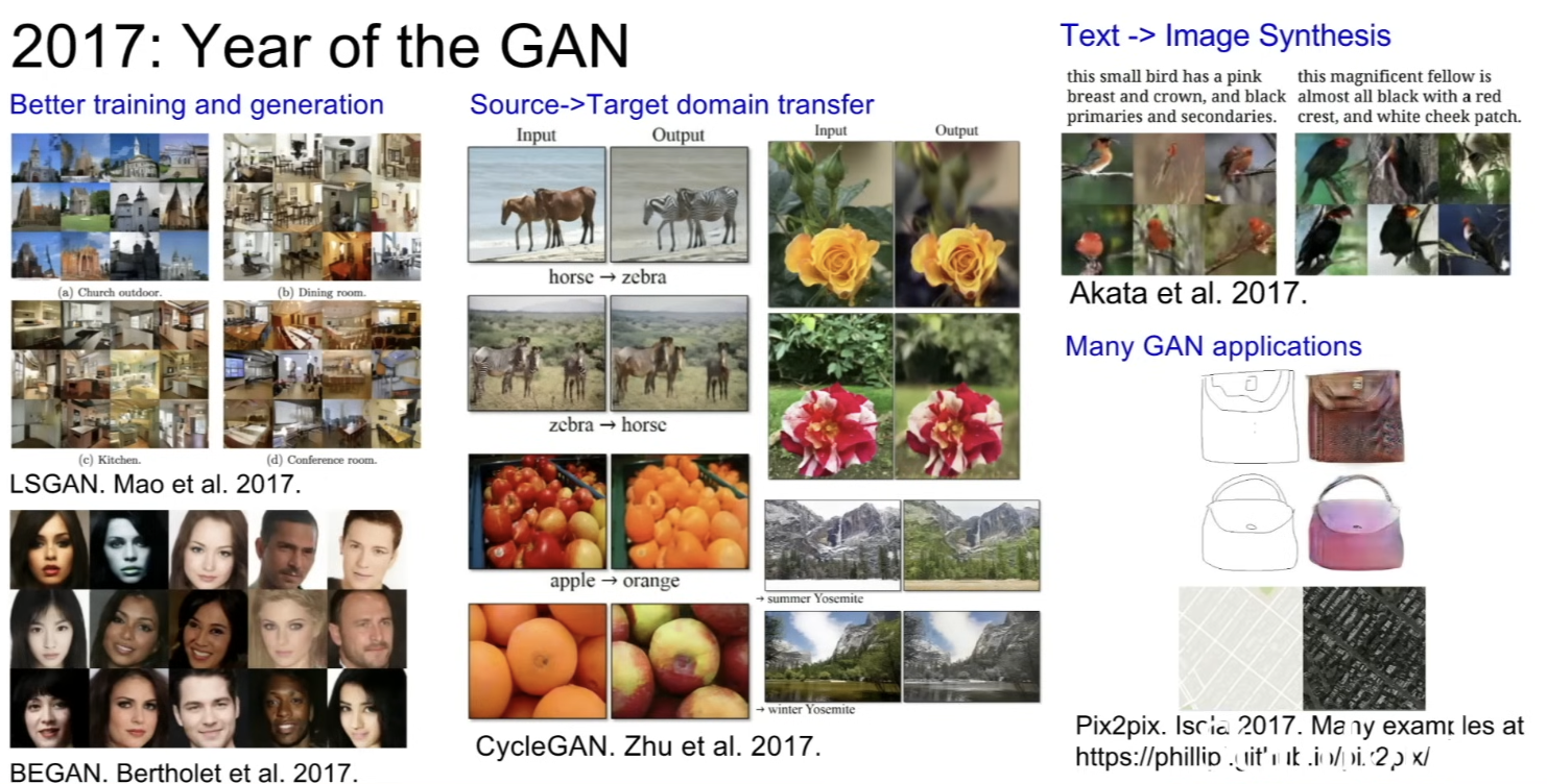
- Conditional GANs, GANs for all kinds of applications
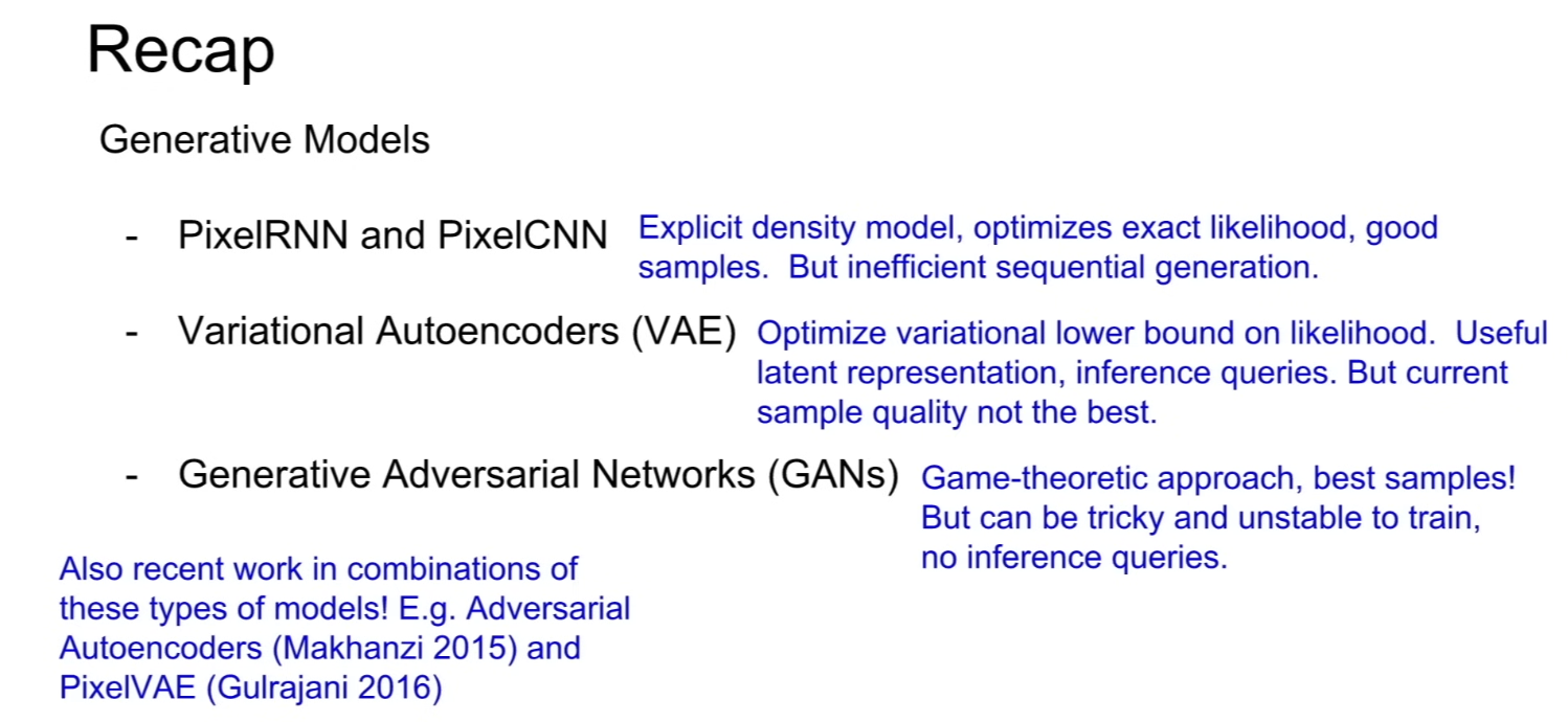
Recap