🔎 Stanford CS231n 강의를 듣고 기록용도로 정리하는 게시글입니다.

AlexNet

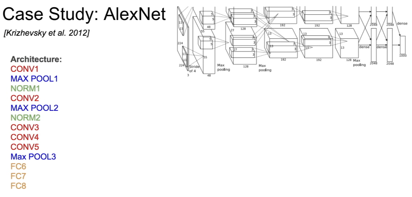
• first large scale convolutional network
  

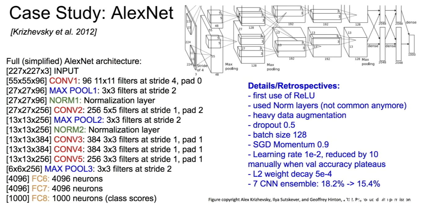
• input: 227x227x3 images (ImageNet)
  

• First layer(CONV1)
  - 96 11x11 filters applied at stride 4

  • Q: Output volume size?
    • size of the output dimension after conv = (227-11)/4 + 1 = 55
    • so, output volume size: 55x55x96 (spatial dimensions at the output = 55x55, and 96 total filters → depth after conv = 96)
  • Q: total number of parameters in this layer?
    • each filter will see through a local region of 11x11x3 (b/c input depth is 3), and there are 96 filters total
    • $\therefore$ 11x11x3x96 = 35k

• Second layer(POOL1)

  • after CONV1: 55x55x96,
  • 3x3 filters applied at stride 2
  • Q: Output volume size?
    • size of the output dimension = (55 - 3) / 2 + 1 = 27
    • so, 27x27x96 (input depth was 96, and pooling preserves depth)
  • Q: Number of parameters in this layer?
    • Nothing!
    • convolutional layers have the weights that we learn, but all we do at pooling is have a rule and look at the pooling region, take the max → no parameters learned

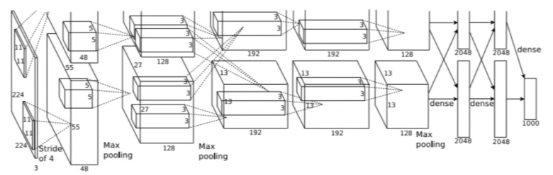
• in AlexNet diagram, it's split into 2 different rows or columns.. going across
  • mostly historical note
  • AlexNet was trained on GTX580 GPUs (old) that only had 3GB of memory ⇒ couldn't actually fit this entire network on here
  • so, they spread the networks across 2 GPUs → on each GPU, have the half of the neurons
  • ex) CONV1 layer - 55x55x96 output, but it's actually split into 48 depth-wise on each GPU
  • CONV1, 2, 4, 5: connections are only with feature maps on the same GPU (so you don't look at the full 96 feature maps)
  • CONV3, FC6, 7, 8: GPUs do talk to each other → there are connections with all feature maps in the preceding layer

VGGNet

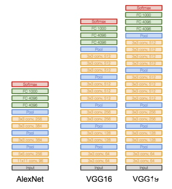
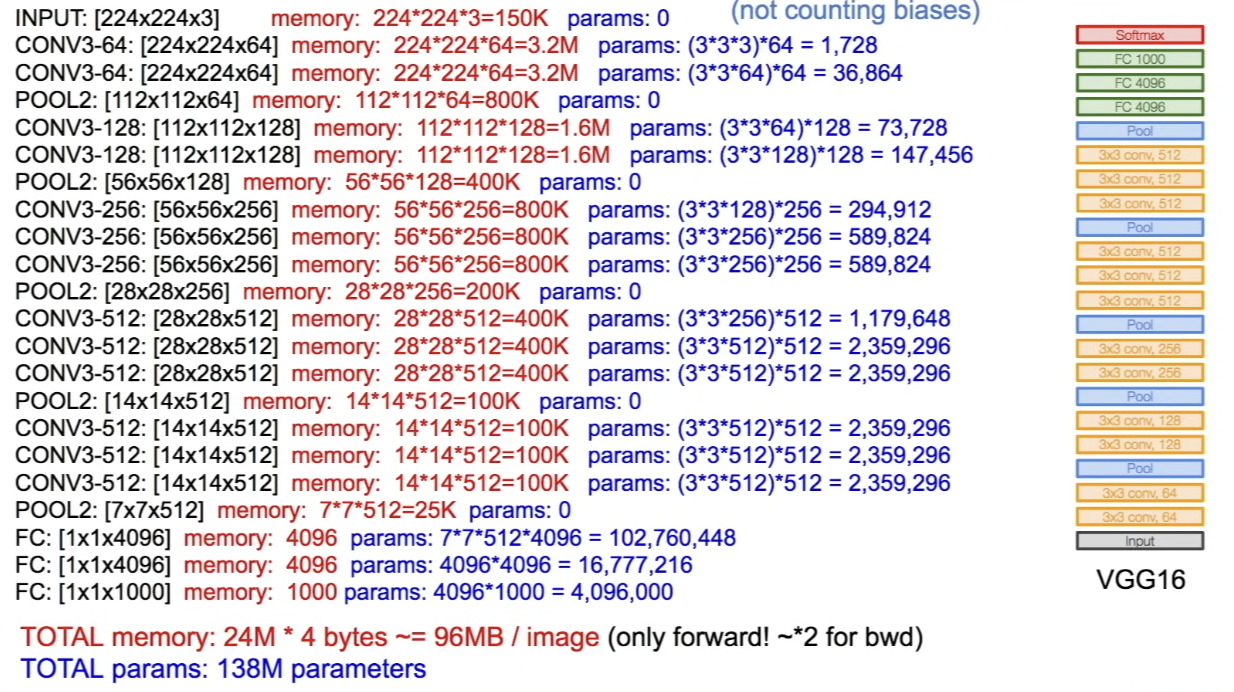
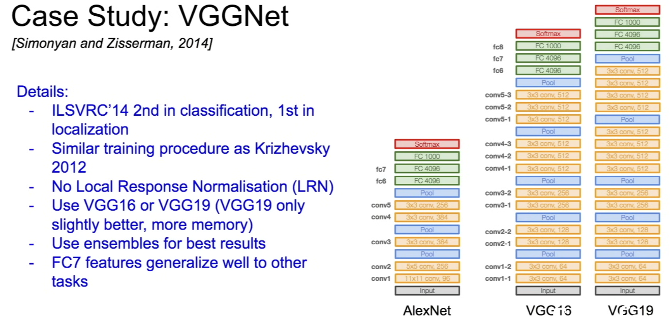
• small filters, deeper networks

• 8 layers(AlexNet) → 16~19 layers in VGGNet

• only 3x3 CONV stride 1, pad 1 and 2x2 MAX POOL stride 2
  

• Q: Why use smaller filters? (3x3 conv)

  • when we take smaller filters, now we have fewer parameters and stack more of them with more depth
  • end up having the same effective receptive field as if you have 1 7x7 conv layer

• Q: What is the effective receptive field of 3 3x3 conv(stride 1) layers?

  • at the 1st layer: receptive field = 3x3
  • at the 2nd layer: each neuron in this layer will look at 3x3 of the 1st layer, but the corners of these 3x3 have an additional pixel on each side that is looking at in the original input layer ⇒ actually looking at 5x5 receptive field
  • at the 3rd layer: this layer looks at 3x3 in the 2nd layer, but is actually looking at 7x7 in the input layer (→ effective receptive field = 7x7)
  • as a result, it's the same as 1 7x7 conv layer
  • but, it's deeper and has more non-linearities, fewer parameters(3x(3x3xCxC) vs. 7x7xCxC for C channels per layer)

Q: Within each layer, what do different filters mean?
A: each filter is a set of weight looking at a 3x3xinput depth → this produces 1 feature map = activation map of all the responses of different spatial locations
- and we can have as many filters as we want, and each of these produces a feature map
- so each filter corresponds to a different pattern we're looking for in the input

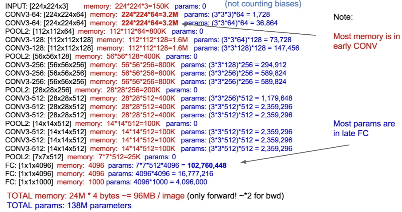
• a lot of memory is in early layers, where you still have large spatial dimensions
• params are usually in the last layers, the FC layers have hugh number of paramters b/c we have dense connections

GoogLeNet

• deeper networks, with computational efficiency
• 22 layers
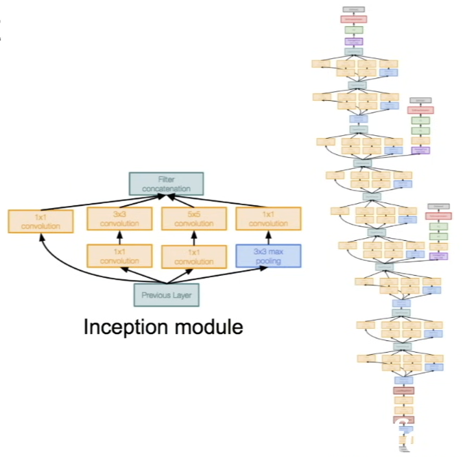
• efficient "Inception" modules
• No FC layers
• Only 5 million parameters (12x less than AlexNet)
• ILSVRC'14 classification winner (6.7% top5 winner)

Inception module

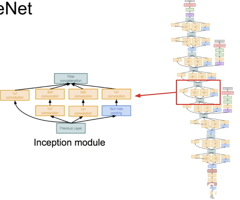
• the idea is to design a good local network topology(체계적인 분류, 위상배치)
• it has the idea of this local topology as a network within a network, and stack a lot of these local topologies on top of each other

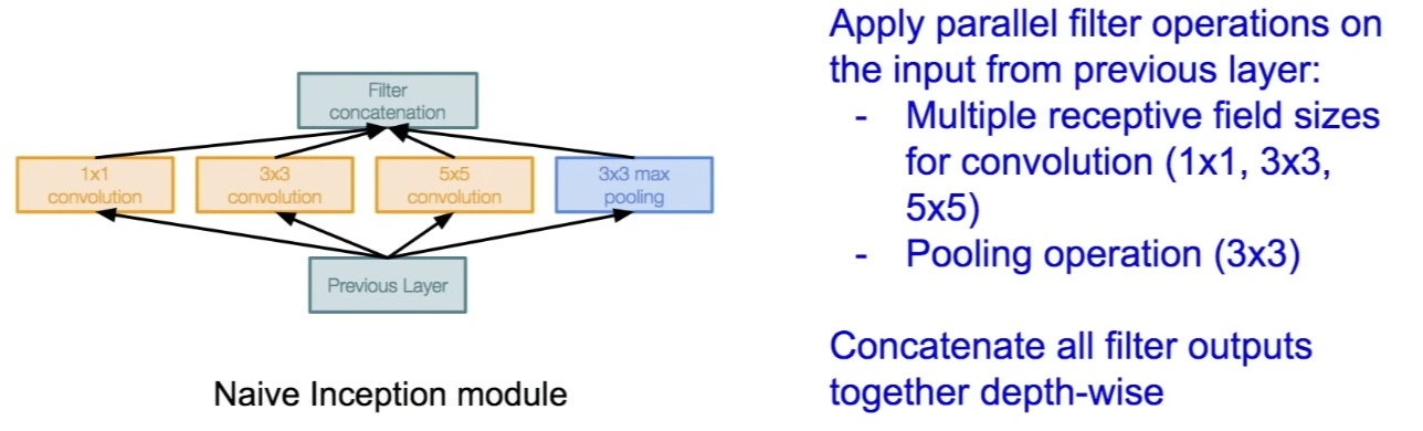
• applying several different kinds of filter operations in parallel on top of the same input coming into this layer

• has input coming in from the previous layer, and do different kinds of convolutions (ex. 1x1 conv, 3x3 conv, 5x5 conv) and pooling operation (3x3)

• so, you get all different outputs from these different layers → concatenate all these filter outputs together depth wise ⇒ creates 1 tenser output at the end (now passes on to the next layer)

• Q: What is the problem with this? (Hint: Computational complexity)
  

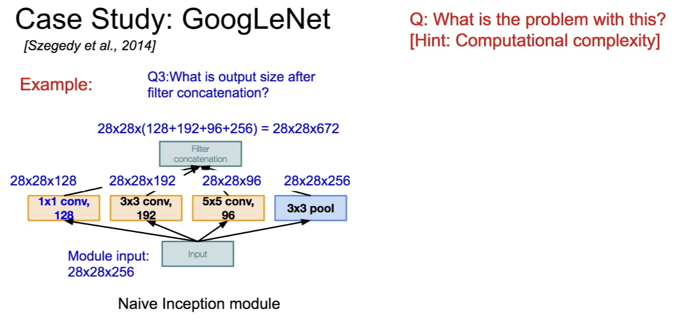
  • consequently, we kept the same spatial dimensions, but blew up the depth
  • (Q: how do we get 28x28 for everything? → A: here we're doing all the 0 padding in order to maintain the spatial dimensions and that way we can do the concatenation depth-wise)
    
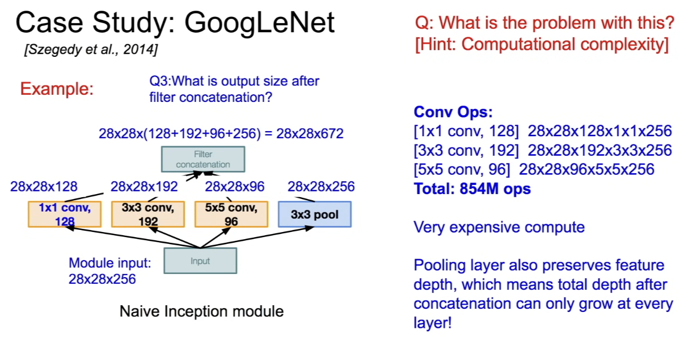
  • for the 1x1 conv, the operations:
    • at each location, we're doing 1x1x256 dot product = 256 multiply operations
    • for each filter map, we have 28x28 spatial locations = 28x28 (the first two numbers)
    • at this layer we have total 128 filters
    • so the total number of these operations = 28x28x128x1x1x256
  • pooling layer also adds to this problem, b/c it preserves the whole feature depth
  • so the depth is increasing as you go up

• Solution: "bottleneck" layers that use 1x1 convolutions to reduce feature depth

  • project these feature maps to lower dimension before convolutional operations(expensive layers) (깊이를 증가시키는 conv 계산을 하기 전에 1x1 conv로 먼저 구조는 유지하되 depth를 감소시킴)
  • idea: 1x1 convolution preserves spatial dimensions, but reduces depth!
    
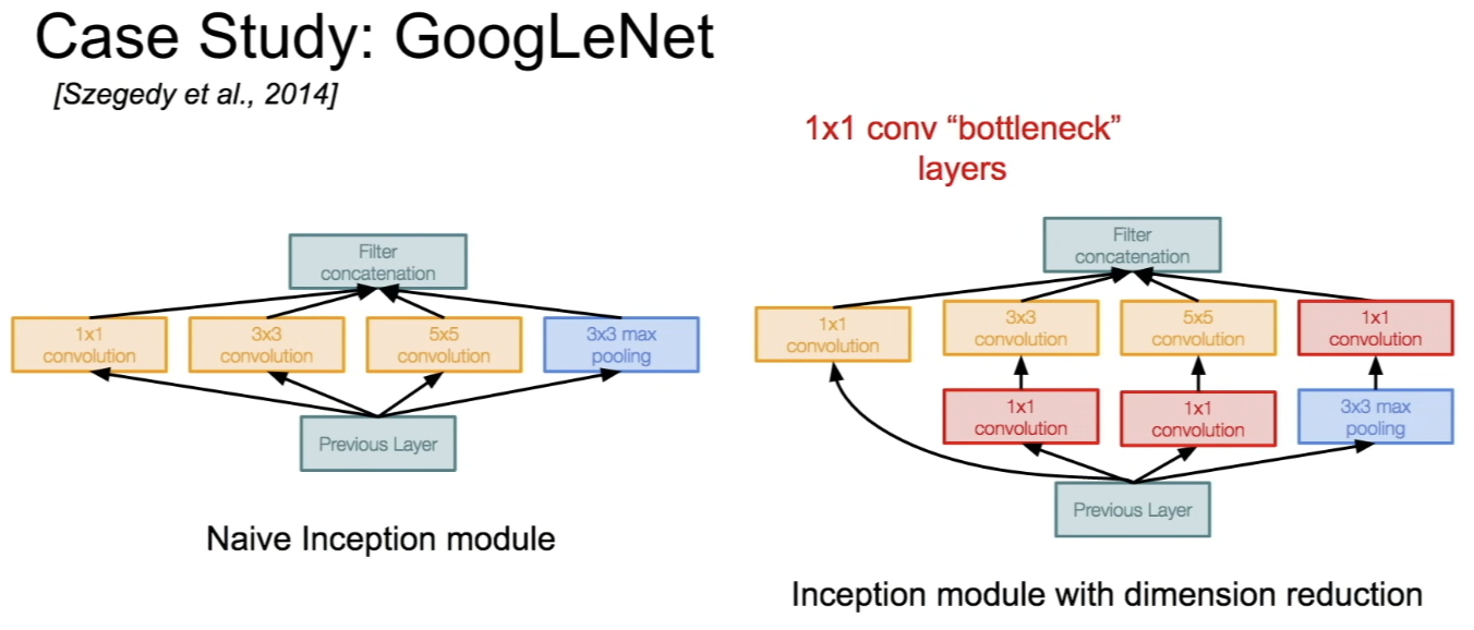
  • so, take the 1x1 convs(= 1x1 conv "bottleneck" layers) and add these at a bunch of places in these modules in order to alleviate(완화하다) this expensive compute

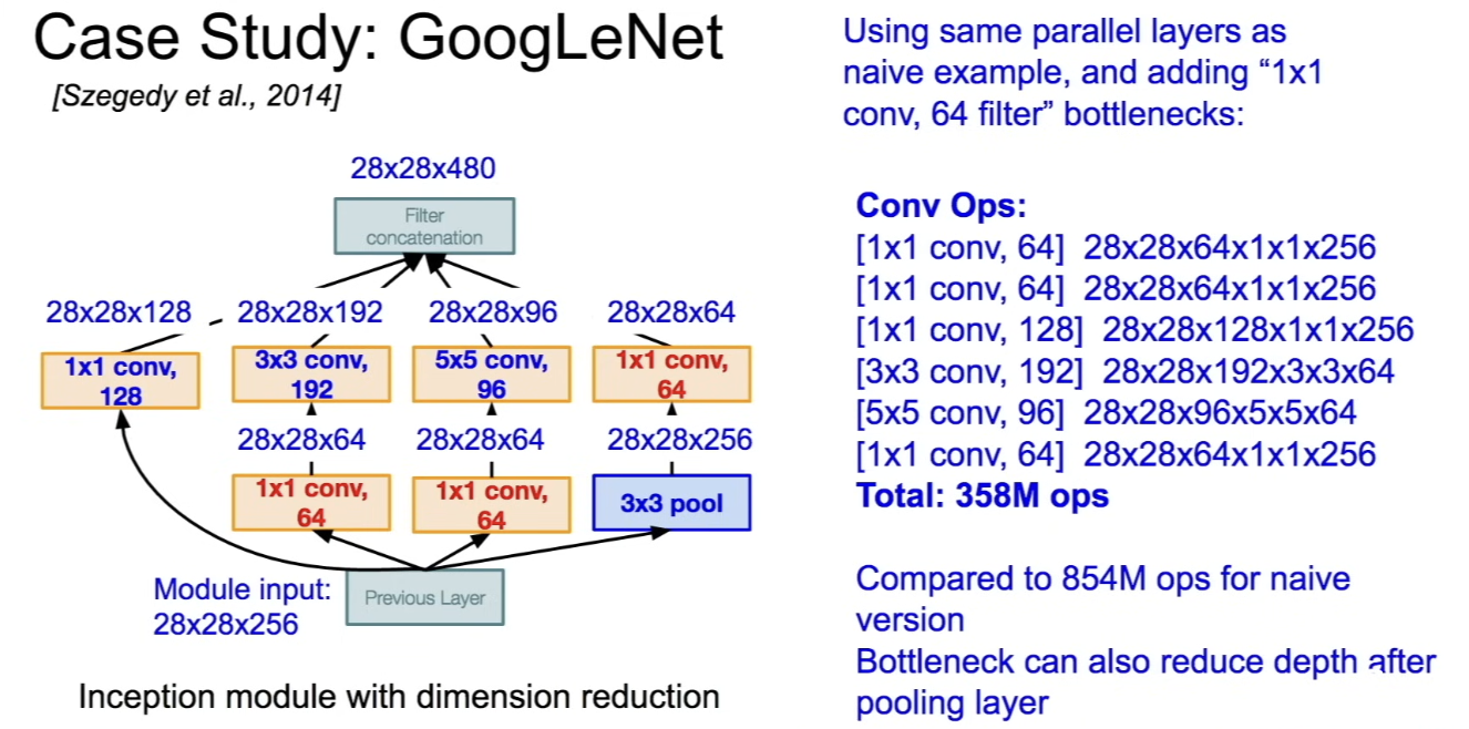
• now, how does this change the math earlier?

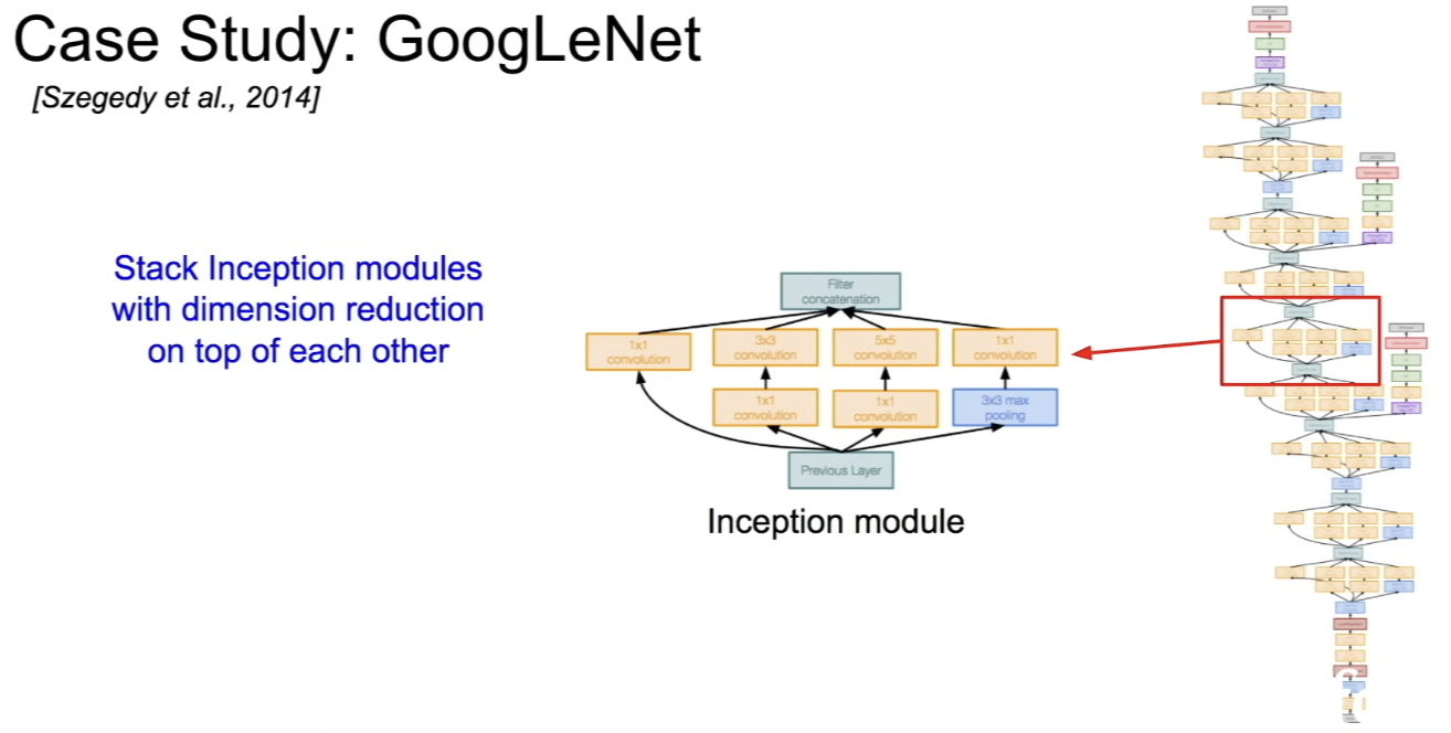
• full inception architecture

---

• flipped version
  

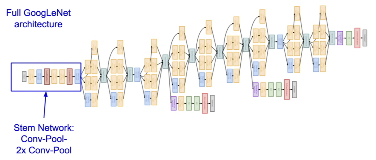
1. stem network - vanilla plain convnet (6 sequence of layers)

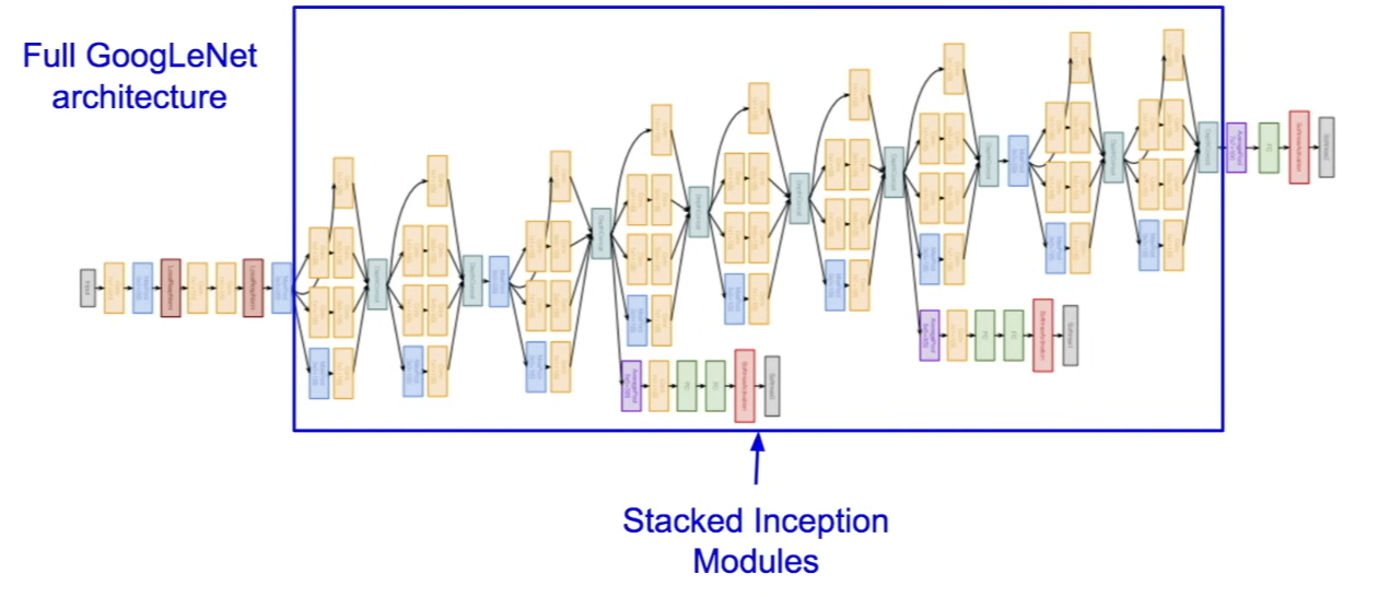
2. multiple inception modules stacked on top of each other

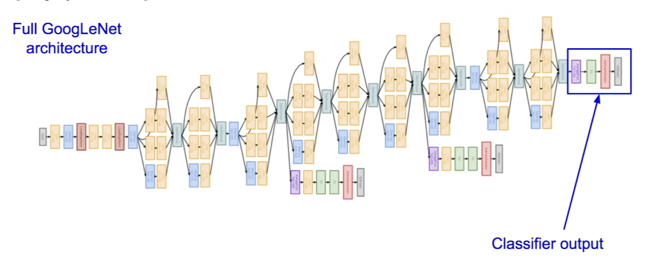
3. classifier output - notice that they removed expensive FC layers, turns out that model works great without them + can reduce parameters

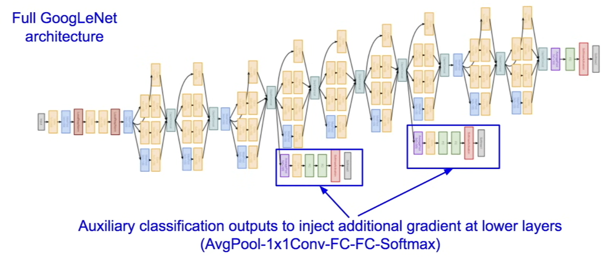
4. extra stems coming out
   • auxiliary(보조의) classification outputs
   • also a little mini network with an average pooling, a 1x1 conv, fc layers, softmax, 1000-way softmax
   • actually using ImageNet training classification loss in 3 separate places (the standard end of the network + 2 places earlier on in the network)
   • reason is that they found out that if you have these auxiliary classification outputs, you get more gradient training injected at the earlier layers, so it's a helpful signal flowing in b/c based off these intermediate layers should also be able to do classification

• total 22 layers with weights(including each parallel layer in an Inception module)

ResNet

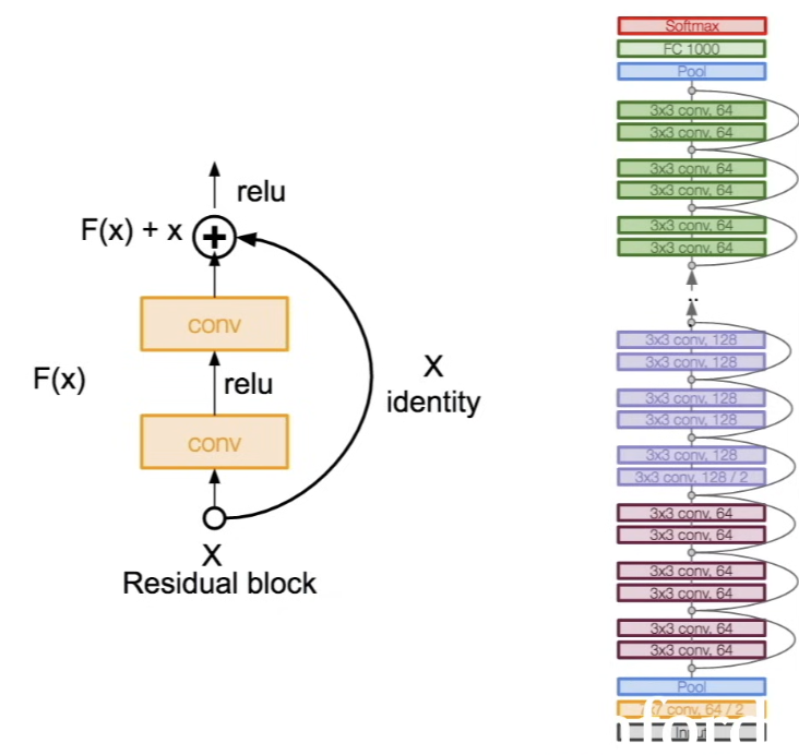
• revolution of depth
• very deep network using residual(잔여의, 잔류의/표본 집단의 회귀식에서 예측된 값 - 실제 관측값) connections
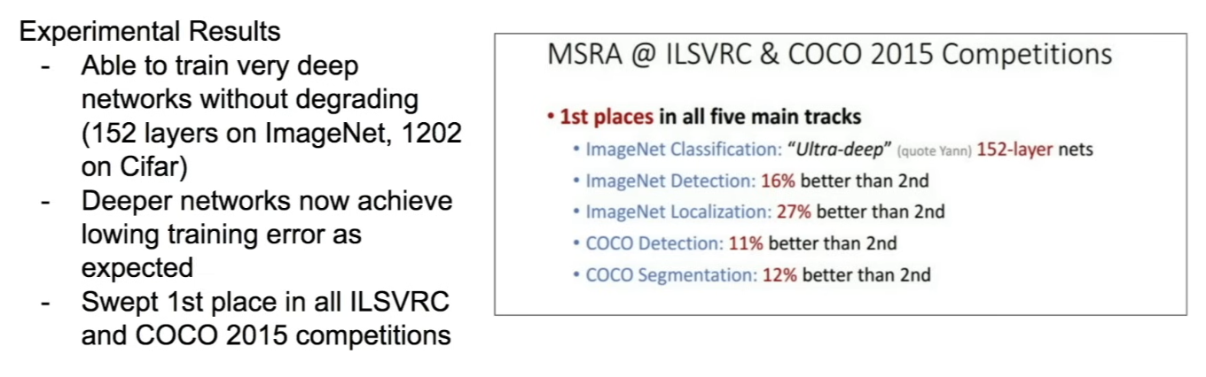
• 152 layer model for ImageNet
• ILSVRC'15 classification winner (3.57% top 5 error)

Idea

• What happens when we continue stacking deeper layers on a "plain" convolutional neural network?
  
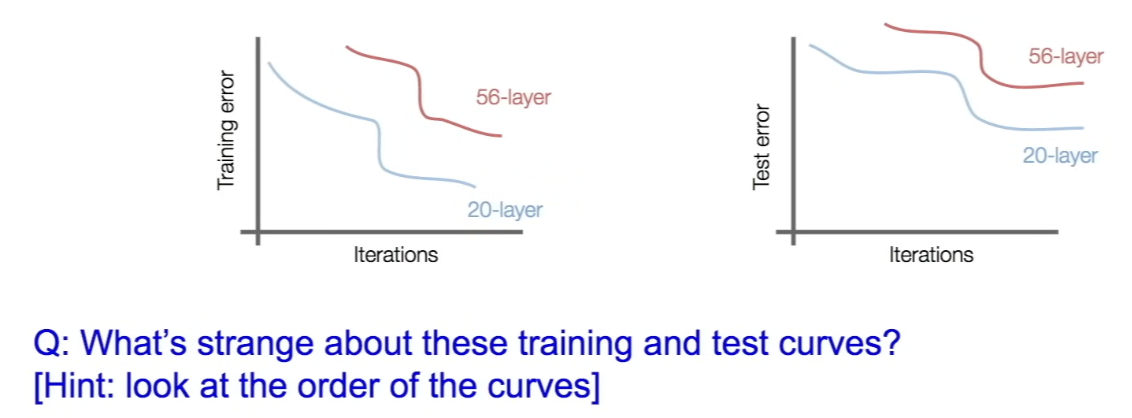
  • in the test error, 56-layer is doing worse than 20-layer network
    ⇒ deeper networks was not able to do better
  • in the training error, we expect for the 56-layer to overfit at some point because it has tons of parameters
    • however, what actually happens is that 56-layer is also doing worse than 20-layer
  • so, even though 56-layer model (deeper) performs worse on both training and test error, this is not caused by overfitting

Hypothesis

• The problem is an optimization problem, deeper models are harder to optimize
  • deeper model should be able to perform at least as well as the shallower model
  • a solution by construction is copying the learned layers from the shallower model and setting additional layers to identity mapping
    • copy the learned layers from the shallower model and for the remaining additional deeper layers, just add identity mapping

Solution

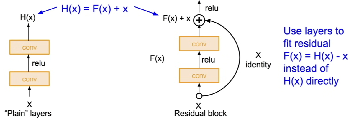
• Use network layers to fit a residual mapping instead of directly trying to fit a desired underlying mapping
  • instead of stacking layers and having every layer try and learn some underlying mapping of a desired function, lets have these blocks where we try and fit a residual mapping (instead of a direct mapping)
  • at the right, input to these block is the input coming in, and use layers to try and fit some residual of desired F(x)-x instead of desired function, F(x)+x
  • at the end of this block, we take the skip connection on the right, this loop, where we take he input and pass it through as an identity
  • so, if we had no weight layers in between, it's going to be identity (same thing as output)
  • but now we use additional weight layers to learn some $\delta$ (=some residual from X)
  • so the output is going to be original X + some residual

Q: What exactly do we mean by residual? (this output of a transformation is residual)
A: We can think of our output as F(x) + x, where F(x) is the output of transformation, and X is input passed through by the identity. Using a plain layer, what we're trying to do is to learn something like H(x), but what we saw earlier was that it's hard to learn a good H(x) as we get very deep networks. So, the idea is to break it down instead of as H(x) = F(x) + x, try and learn F(x). Instead of learning H(x) directly, learn what it is that we need to add or subtract to our input as we move on the next layer. So, 'residual' = F(x)

Full Architecture

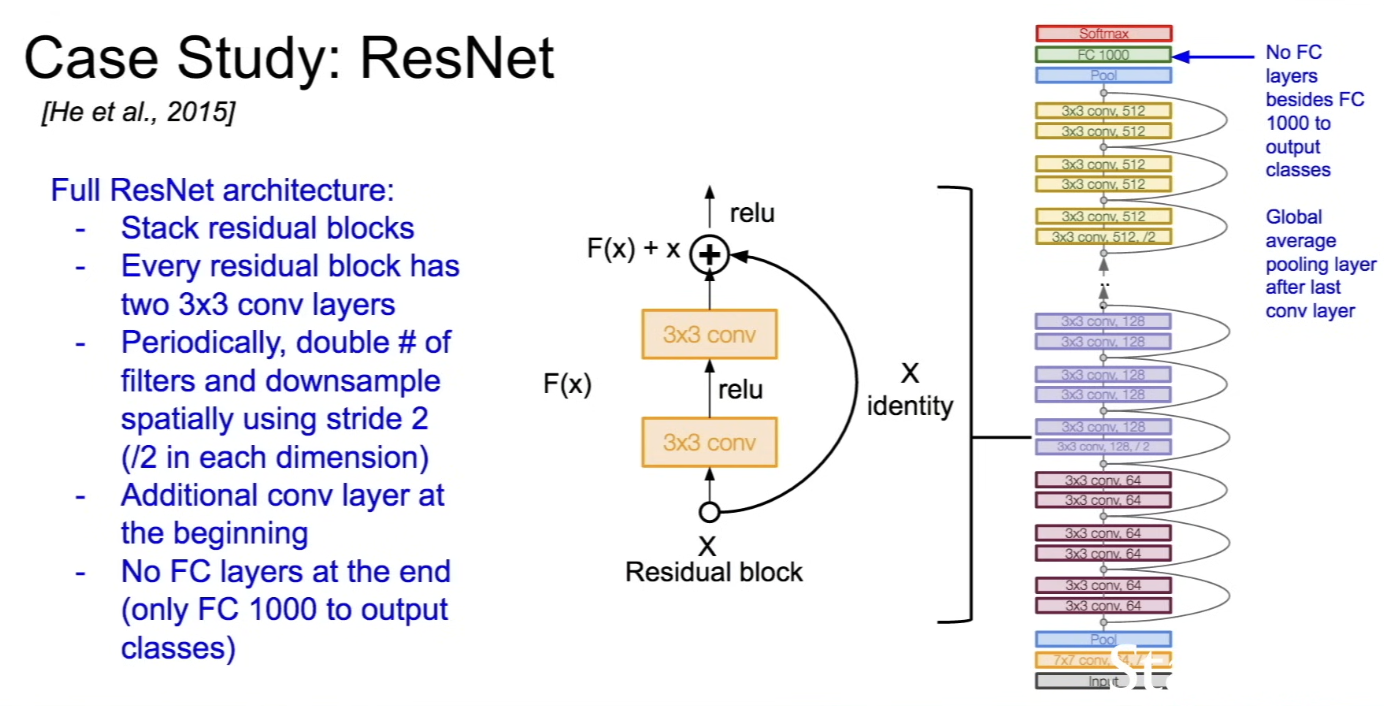
• total depths of 34, 50, 101 or 152 layers for ImageNet

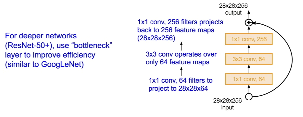
• for very deep networks(for ones that are more than 50 layers deep), they also use bottleneck layers (similar to what GoogleNet did in order to improve efficiency)

• within each block, have 1x1 conv filter that projects it down to a smaller depth

• Training ResNet in practice:

  • Batch Normalization after every CONV layer
  • Xavier/2 initialization from He et al.
  • SGD + Momentum(0.9)
  • Learning rate: 0.1, divided by 10 when validation error plaeteaus
  • Mini-batch size 256
  • Weight decay of 1e-5
  • No dropout used

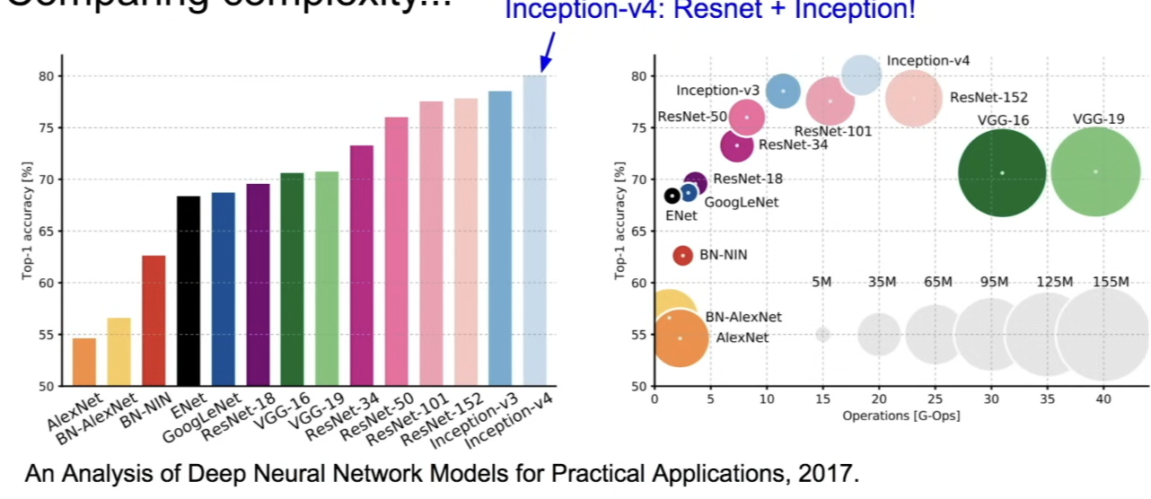
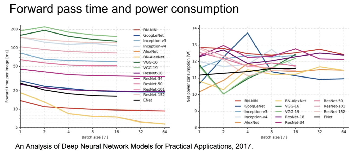
Comparison

Other architectures to know

NiN (Network in Network)

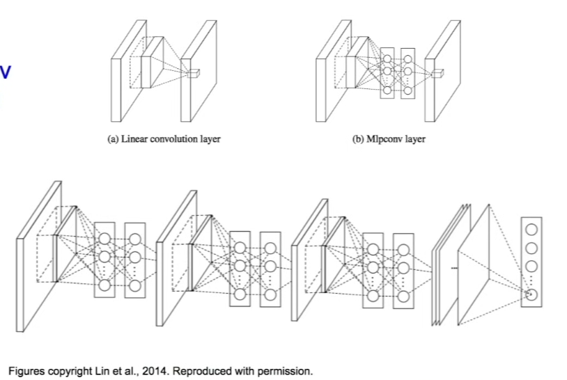
• from 2014
• Mlpconv layer with "micronetwork" within each conv layer to compute more abstract features for local patches
  - within each conv layer, trying to stack an MLP with a couple of FC layers on top of the standard conv and be able to compute more abstract features for these local patches
• Micronetwork uses multiplayer perceptron (FC, i.e. 1x1 conv layers)
• Precursor to GoogLeNet and ResNet "bottleneck" layers
• Philosophical inspiration for GoogLeNet

Improving ResNets...

Identity mappings in deep Residual Networks

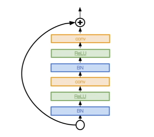
• Improved ResNet block design from creators of ResNet
• Creates a more direct path for propagating information throughout network (moves activation to residual mapping pathway)
  - adjusted layers that were in the ResNet block path
  • a good path to propagate information all the way up, and then backprop all the way down again
• Gives better performance

Wide Residual Networks

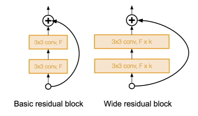
• Argues that residuals are the important factor, not depth
  - ResNets made networks much deeper as well as added these residual connections
• User wider residual blocks (F x k filters instead of F filters in each layer)
  - wider = more filters in conv layer
• 50-layer wide ResNet outperforms 152-layer original ResNet
• Increasing width instead of depth more computationally efficient (parallelizable)

ResNeXT (Aggregated Residual Transformations for Deep Neural Networks)

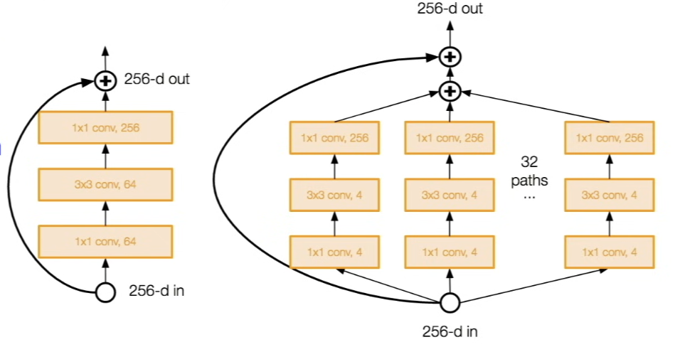
• Also from creators of ResNet
• Increases width of residual block through multiple parallel pathways ("cardinality" = total number of those pathways)
  - instead of increasing the width of the residual block through more filters
• parallel pathways similar in spirit to Inception module

Deep Networks with Stochastic Depth

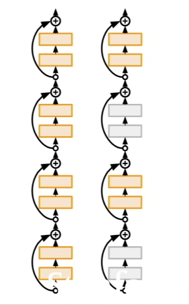
• Motivation: reduce vanishing gradients and training time through short networks during training
  - looking more at the depth problem
  • once you get deeper and deeper, the typical problem is vanishing gradients (gradients will get smaller and eventually vanish as you're trying to backpropagate them over very large number of layers)
• Randomly drop a subset of layers during each training pass
• Bypass with identity function
• Use full deep networks at test time

FractalNet

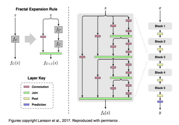
• Ultra-Deep Neural Netowrks without Residuals
• Argues that key is transitioning effectively from shallow to deep and residual representations are not necessary
• Fractal architecture with both shallow and deep paths to output
  - different length pathways
• Trained with dropping out sub-paths
• Full network at test time
  - was able to get a good performance

DenseNet

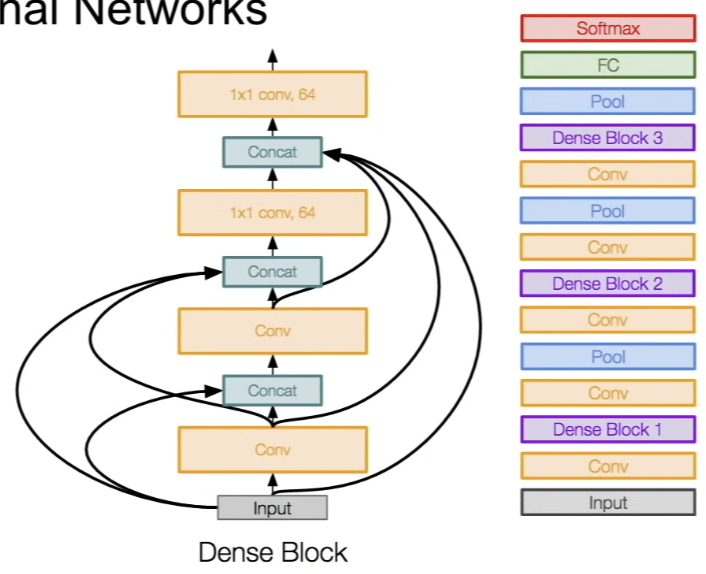
• Densely Connected Convolutional Networks
• Dense blocks where each layer is connected to every other layer in feedforward fashion
  - input to the block is also the input to every other conv layer
  • as you compute each conv output, those outputs are now connected to every layer after it
  • these are all concatenated as input to the conv layer, and they have other processes for reducing the dimensions and keeping efficient
• Alleviates vanishing gradient, strengthens feature propagation, encourages feature reuse

SqueezeNet

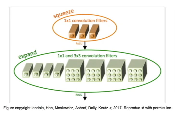
• AlexNet-level accuracy with 50x fewer parameters and <0.5Mb Model Size
• Fire modules consisting of a 'squeeze' layer with 1x1 filters feeding an 'expand' layer with 1x1 and 3x3 filters
• AlexNet level accuracy on ImageNet with 50x fewer parameters
• Can compress to 510x smaller than AlexNet (0.5Mb)
• direction of how do we have efficient networks model compression...