🔎 Stanford CS231n 강의를 듣고 기록용도로 정리하는 게시글입니다.

• 저번 시간에 W를 어떻게 선택할지에 대해 얘기하지 않음
• 실제로 어떤 W값이 최선일지에 대해, 또 training data를 어떻게 사용해야 하는지에 대해

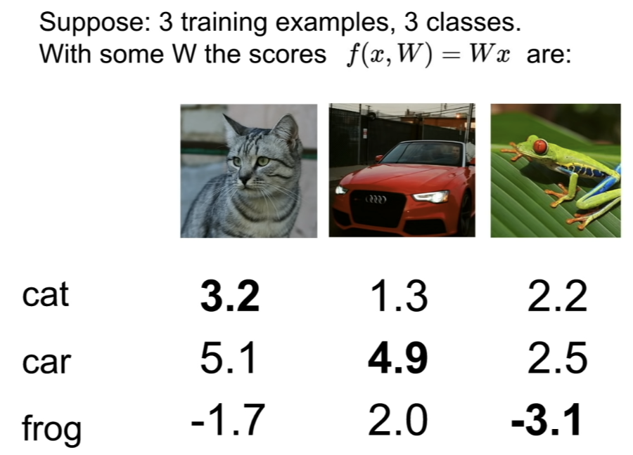
• in this case, cat is not correctly classified, car is, but frog score is wrong

Loss Function

• 이 classifier가 얼마나 잘 작동하는지를 알려주는 함수
  • given a dataset of examples ${(x_i, y_i)}_{i=1}^N$, where $x_i$ is image, $y_i$ is (integer, in this case, it's score) label
  • $\displaystyle L = \frac{1}{N}\sum_iL_i(f(x_i, W), y_i)$
  • $L_i$ is loss function
    • input: predicted score from function f, true target label y
    • output: quantative value for how bad the predictions are for the training example
  • $L$ is average of losses

Multiclass SVM loss

• unlike SVM, it handles multiple classes
• sums over all of the categories ($Y$) except for the true category $Y_i$
  $\displaystyle \begin{aligned}L_i & = \sum_{j \neq y_i} \begin {cases} 0 & \text{if }s_{y_i} \gt s_j + 1 \\ s_j-s_{y_i}+1 & \text{otherwise} \end{cases} \\ & = \sum_{j \neq y_i} max(0, s_j-s_{y_i}+1)\end{aligned}$
  • compare the score of the correct category and the incorrect category
    • if score for the correct category > score for the incorrect category → $loss = 0$
      ⇒ sum these up over all incorrect categories
• scores vector: $s = f(x_i, W)$, SVM loss form is the following:

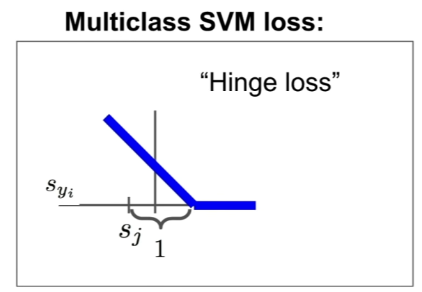
• 어떤 값과 0 사이의 max값을 취하는 형식의 loss function은 hinge loss임
• x축: $s_{y_i}$ = score for true category
• y축: $loss$
• $s_{y_i}$가 증가할수록, 어떤 safety margin에 도달하기까지 loss가 선형적으로 감소하고, 그 이후에는 correctly classified했으므로 $loss = 0$
• 이 loss값이 궁극적으로 말해주는 것은 정답인 카테고리에 대한 점수가 다른 점수들보다 크면 happy하다는 것임

Calculating Multiclass SVM loss for those 3 examples

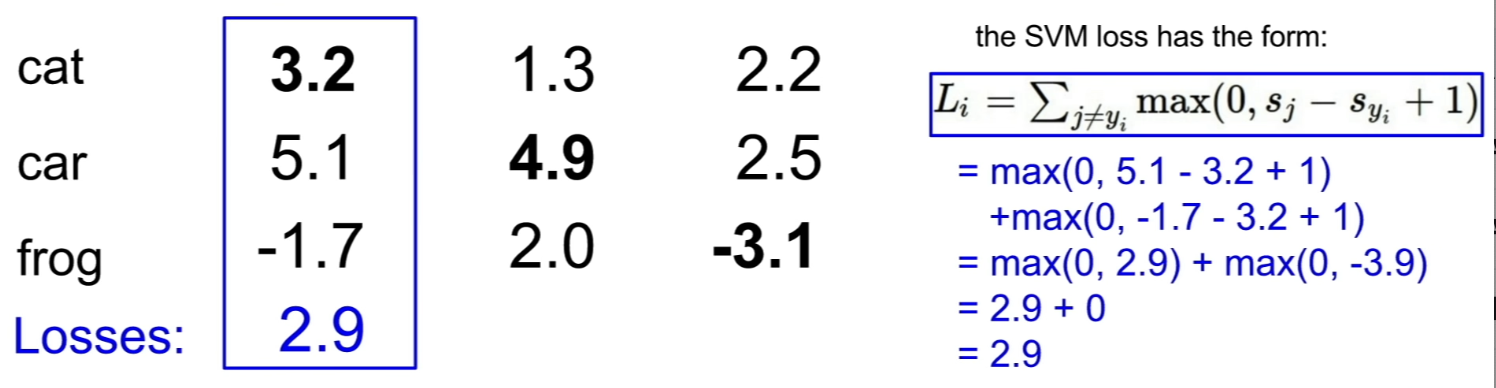
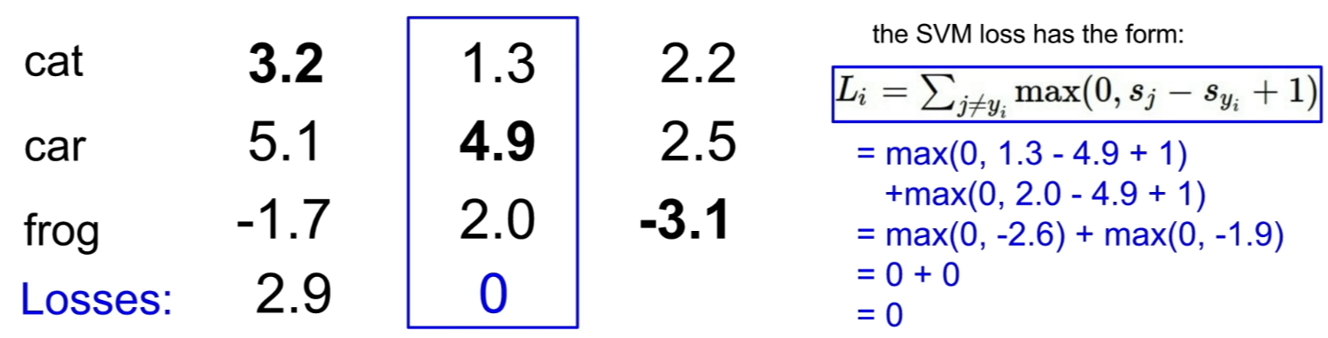
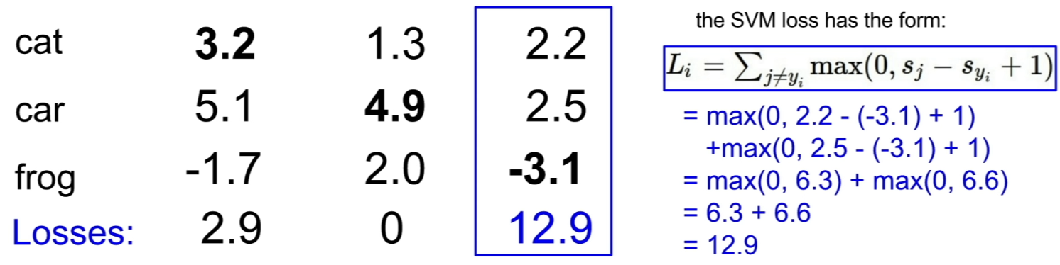
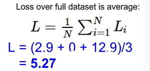
• 결과적으로, 여기에서 사용한 classifier는 이 data set에 대해 5.3만큼이나 좋지 않음

Q: How do you choose "plus one"?
A: We don't actually care about the "absolute" values of the scores in this loss function, only care about the relative differences between the scores, only care that the correct score is much greater than the incorrect score. So, the choice of 1 doesn't matter. Later on, the "1" is canceled with the overall setting of the scale in $W$.

Some Questions

1. If car scores change a bit, what happens to loss?
   • Nothing.
   • SVM loss only cares about getting the correct score to be greater than one more than the incorrect scores
   • But in this case, the car score is already quite a bit larger than the others, and this margin of the '1' will still be retained, so the loss will not change.
2. What is the min/max possible loss?
   • minimum loss = 0 (if our correct scores were much larger, all of the loss will be 0)
   • maximum loss = $\infty$ (if the correct score goes very negative, we could incur potentially infinite loss)
3. At initialization, W is small, so all s is approximately 0. What is the loss?
   • number of classes - 1
   • We're looping over C-1 classes, the two $S$s will be about the same, which means $max(0, 1) = 1$ → so we'll get C-1

⇒ this is useful debugging strategy. when you start training, you should think about what you expect your loss to be, and if the loss you actually see at the start of training at that first iteration is not equal to C-1, means you probably have a bug

4. What if the sum was over all classes? (including $j = y_i$)
   • (originally, SVM sums up scores over the incorrect scores)
   • loss increases by 1
5. What if we used mean instead of sum?
   • nothing changes; number of classes is fixed ahead of time, so that's just rescaling the whole loss function by a constant, so it doesn't really matter
6. What if we change the loss formulation to $L_i = \sum_{j\neq y_i} max(0, s_j-s_{y_i}+1)^2$
   • this would be a different classification algorithm
   • here, we're changing the trade-offs between good and badness in kind of a nonlinear way, so we'll end up computing a different loss function
   • this method gets used sometimes in practice. it means that things that are bad gets squared bad = even more bad → whereas, if you're using hinge loss, we don't care being a little bit wrong and a lot wrong.

Multiclass SVM Loss: Example Code

def L_i_vectorized(x, y, W):
	scores = W.dot(x)
    margins = np.maximum(0, scores - scores[y] + 1)
    margins[y] = 0
    loss_i = np.sum(margins)
    return loss_i

Is a W that makes L = 0 unique?

• no. there are other $W$s.
• $2W$ also makes $L = 0$. it's because margins between the correct and incorrect scores will also double = all these margins were already greater than 1 and we double them, it'll be still greater than 1, so we still get 0 loss.

Regularization

Why do we need it

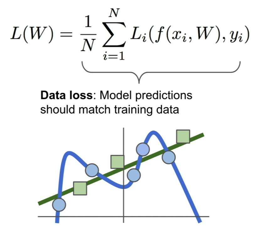
• the loss function above makes the classifier "fit" the training data
  • however, we don't actually care about training data performance, we care about performance on test data
• if we have the new data(green) come in, the blue line is going to be totally wrong
• what we would have preferred the classifier to do was the strict green line
  • rather than blue line that perfectly fits the training data
• this is a core fundamental problem in machine learning, and we solve it by regularization

Regularization

• add an additional term to the loss function
• in addition to data loss(which will tell our classifier that it should fit training data), we'll add another term which encourages the model to somehow pick the simpler $W$. ("simple" depends on the task and the model)
• whole idea is from Occam's Razor
  -"Among competing hypotheses, the simplest is the best"

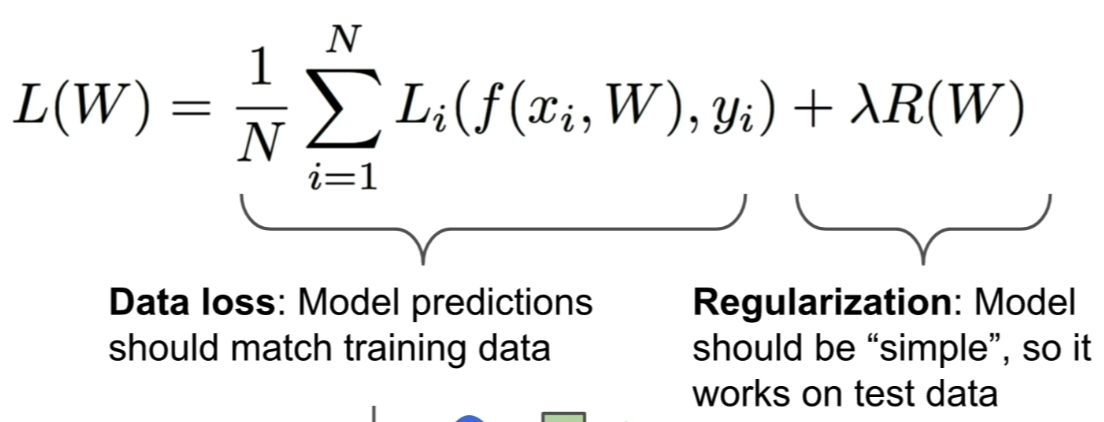
• standard loss function has two terms; data loss, regularization loss, hyper-parameter(lambda - trades off between the two)

Types of Regularization

1. L2 Regularization(Weight Decay)

• euclidean norm of $W$(weight vector)
• penalizing the euclidean norm of this weight vector
  
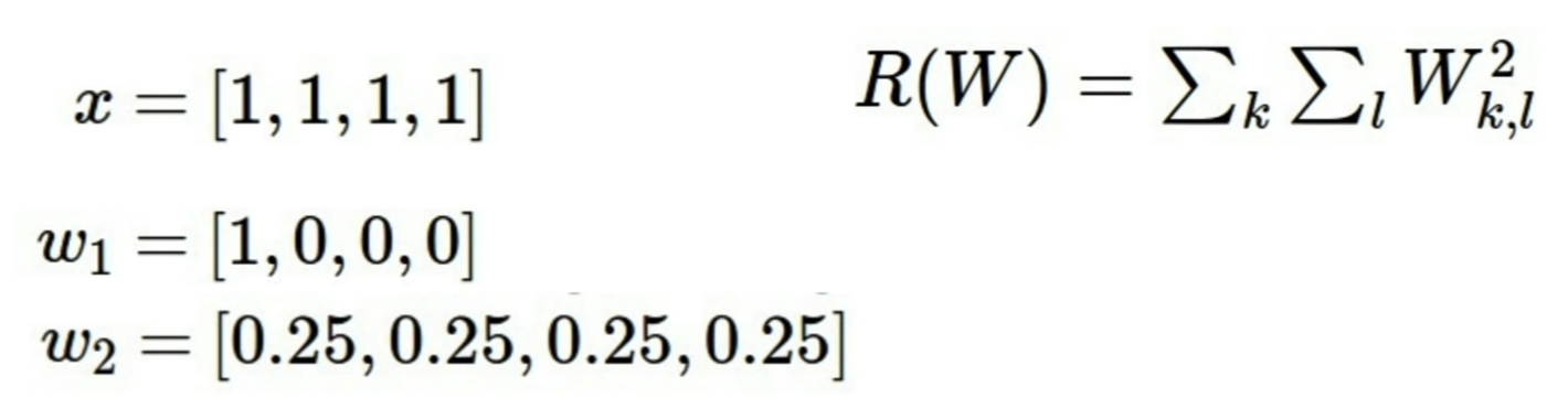
  • we're considering two different possibilities for W
  • when we're doing linear classification, we're doing dot products between our $x$ and $W$, these two $W$s are the same b/c they give out the same result when dot producted with $x$
  • which one would L2 regression prefer? → $W2$, b/c it has a smaller norm(벡터의 길이)
  • L2 regression measures complexity of the classifier in a relatively coarse(거친) way
  • L.C has interpretation of how much the value of the vector $x$ corresponds to the output class, so the L2 regularization is saying that it prefers to spread that influence across all the different values in $x$

2. L1 Regularization

• penzalizing the L1 norm of the weight vector
• has properties that encourage sparsity(희박, 성김, 희소) in $W$
• opposite interpretation compared to L2 regularization
  • would prefer W1 over W2
    • bc L1 reg has different notion of complexity
      • saying that maybe the model is less complex if the weight vector has less 0s, so the question of how do we measure complexity and how does L2 measure complexity is problem dependent, so you have to think about the particualr setup and data, and think about how the complexity should be measure on this task
        - (위의 경우 L1 = L2이긴 하지만)

3. Elastic net(L1 + L2)
4. Max norm regularization
5. Dropout
6. Batch normalization, stocahstic depth

• whole idea of regularization is that any thing that you do to your model that penalizes somehow the complexity of the model rather than explicitly trying to fit the train data

Softmax loss (Multinomial Logistic Regression)

• another popular choice for loss function in DL

• in Multiclass SVM, we didn't have interpretation for the scores

• for multinomial logistic regression, endow(기부하다) scores with some additional meaning, and use the scores to compute probability distribution over classes

  • scores = unnormalized log probabilities of the classes

• we use softmax function

  • take all of our scores,
  • exponentiate them(become positive),
  • re-normalize them by the sum of those exponents

• send scores to the softmax function, end up with this probability distribution, and we have probabilites over our classes, and the sum of probabilities across all the classes sum to 1
  $\displaystyle P(Y=k|X=x_i) = \frac{e^{s_k}}{\sum_je^{s_j}} \ \text{where} \ s = f(x_i,W)$

• the interpretation is that we want to compare the computed probability distribution implied by scores and the target(true probability distribution)

• want to encourage the computed probability distribution from softmax function to match the target probability distribution that has all the mass on the correct class(e.g. if it's cat, we want probability for cat to be 1)

  • softmax 계산 결과 나온 확률 분포가 정답의 확률 분포를 따르는 것이 목표?

• What we want is the probability of the true class to be high and as close to 1

• loss will be the negative log of the probability of the true class
  $L_i = -logP(Y=y_i|X=x_i)$

  • 로그를 쓰는 이유는 원래 값 (raw probability)보다 로그 값을 최대화하는 것이 수학적으로 쉽기 때문임
  • 로그는 증가만 함(monotonic) → 정답일 확률의 log값을 최대화한다 = badness를 측정하는 값을 최대화한다 → 앞에 - 를 붙임

• in summary, $\displaystyle L_i = -log(\frac{e^{s_{y_i}}}{\sum_je^{s_j}})$

Example

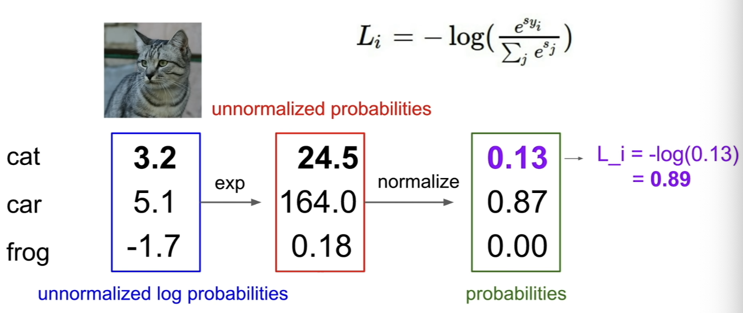
• 3 scores that came out of our linear classifier = exactly the way that they were in the context of SVM loss
• rather than taking these scores and putting them directly into the loss function, exponentiate all of them(so that they're all positive) → normalize them(to make sure they all sum to 1) → loss will the minus log of each value

1. What is the min/max value of the softmax loss?
   • min = 0 (theoretically)
     • probability distribution that we want is 1 on the correct class, 0 on the incorrect classes
     • if that were the case, inside the log will be 1 and $-\log1 = 0$, loss would be 0
     • in order to get the thing totally right, our scores would have to look like infinity score for the correct class, -infinity score for all the incorrect classes (b/c we do exponentiation and normalization)
     • but computers don't deal with infinities, so in practice you'll never get 0 loss
   • max = $\infty$
     • suppose that we have 0 probability on the correct class, $-\log0 = \infty$
     • but, you'll never get here b/c the only way you can get this probability to be 0 is..
       • if $e^{\text{correct class score}} = 0$, and it can only happen if the correct class score is $-\infty$
2. Usually at initialiation W is small, so all s is approximately 0. What is the loss?
   • $\log C$

Comparing the two loss functions

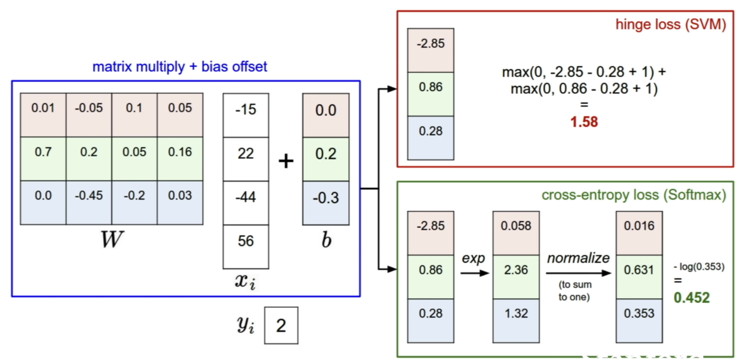
• linear classification

  • $W$ gets multiplied against our input to produce scores

• difference = how we choose to interpret those scores to quantitatively measure the badness afterwards

  • SVM - look at the margins between the scores of the correct class and incorrect classes
  • softmax - compute a probability distribution, and look at the -log probability of the correct class

• in multi-class SVM loss, when the car score was much better than all the incorrect scores, jiggling the scores for that car image didn't change the loss at all

  • b/c the only thing that SVM loss cares about is getting that correct score to be greater than a margin above the incorrect scores

• BUT softmax is different

  • always wants the probability mass all the way to 1
  • so even if you're giving high score to correct score, softmax will want to continue pushing that score of the correct class up toward $\infty$, and the score of the incorrect classes down toward $-\infty$

Recap

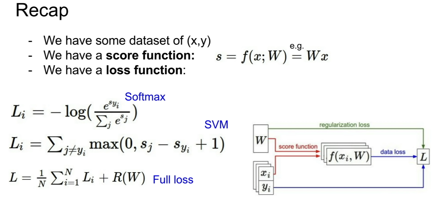
Optimization

• In practice, once your prediction function $f$, loss function, regularizer gets big and complex, there's not much hope in trying to write down an explicit analytic solution that takes you directly to the minima
• In practice, we use iterative methods where we start with some solution and gradually improve it over time

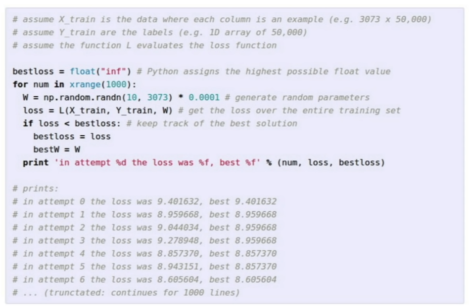
Strategy 1. Random Search

• Take a bunch of $W$ sampled randomly, throw them into loss function and see how well they do

• really bad algorithm, should not use this
  
  

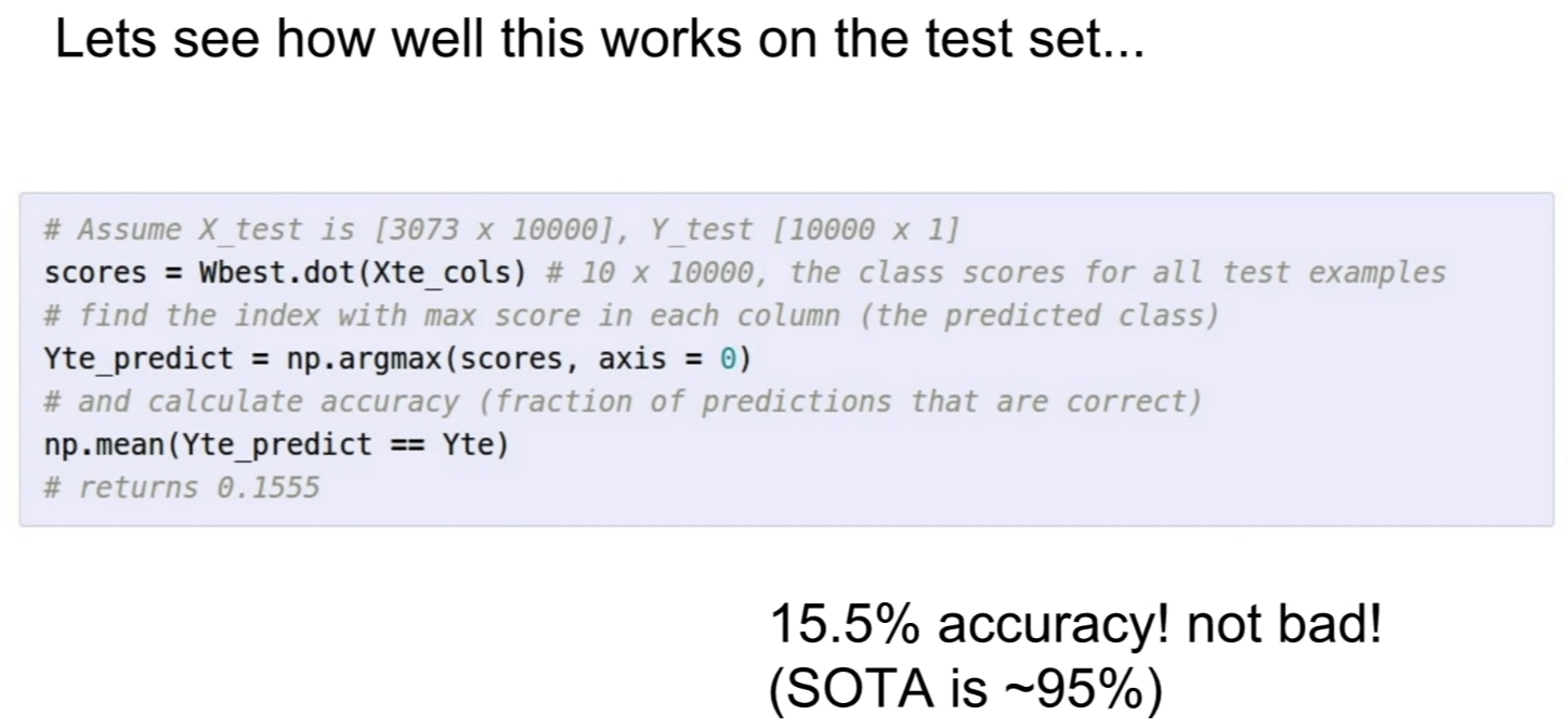
• random chance is 10%, and if we did random trials, some setting $W$ got 15% accuracy → better than random, but state of the art is 95%, got a gap to close

Strategy 2. Follow the slope

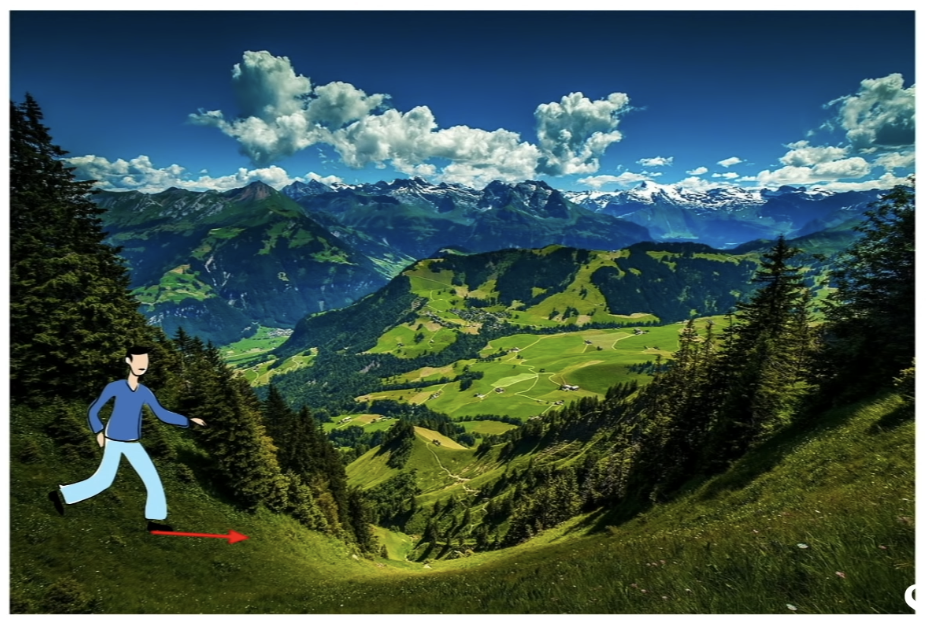
• using the local geometry of this landscape

• you can determine which way would take you a little down the hill

• repeat, and hope that you'll end up at the bottom of the valley eventually

• tends to work really well in practice

  • generally the strategy when training linear classifier, neural network and other things

• in 1-D, slope = derivative(미분, 도함수) of this function
  = $\displaystyle\frac{df(x)}{dx} = \displaystyle\lim_{h\rarr0}\frac{f(x+h)-f(x)}{h}$

Gradient

• gradient is the vector of (편미분) along each dimension
  • generalization of derivative in multi variable setting
  • each element of the gradient tells us what the slope of the function $f$ is, if we move in that coordinate direction
    • = how much the loss will change if we move a tiny amount in that coordinate direction
  • gradients point in the direction of greatest increase of the function
    • if you look at the negative gradient direction, it gives you the direction of the greatest decrease of the function
  • generally, slope of the landscape in any direction = the dot product of the gradient with the unit vector describing that direction
• a lot of DL is about computing gradients of your functions, and using those gradients to iteratively update your parameter vector

Evaluating gradient

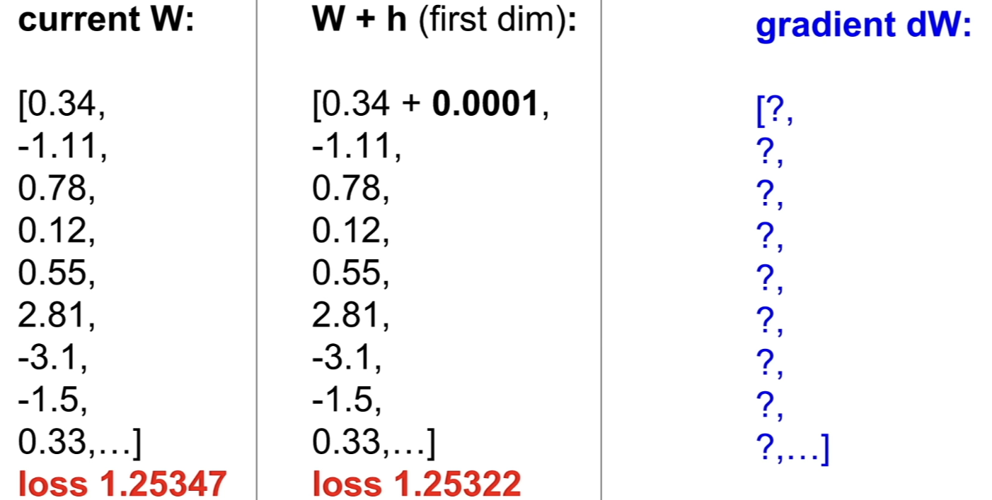
• using the method of finite differences(going back to the limit definition of gradient)
  

• ex) increment the first element of $W$ by a small value $h$ and recompute the loss

  • loss would decrease a little bit

    

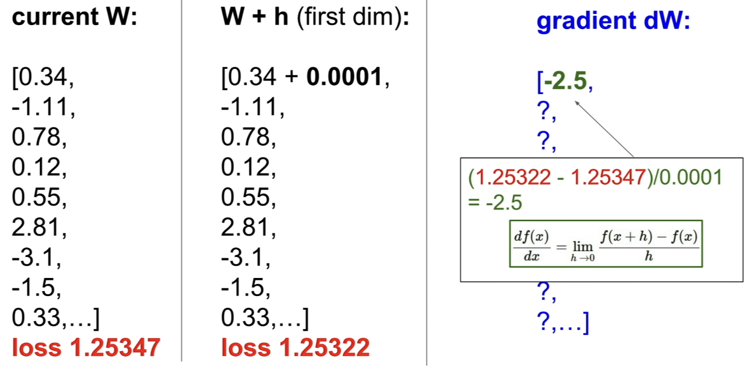
  • then, use the limit definition to come up with the finite differences approximation to the gradient in this first dimension

  • repeat the procedure in the second dimension,

    

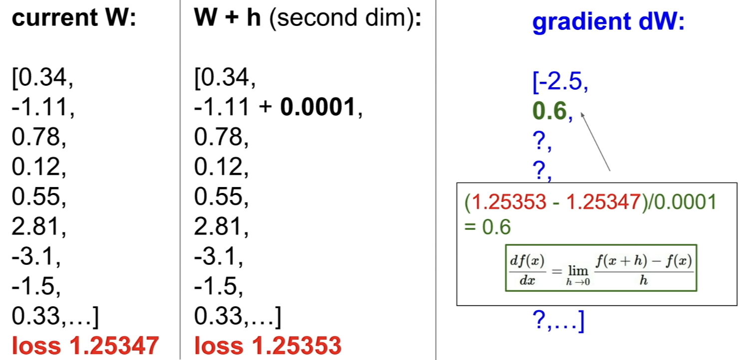
• this is a terrible idea b/c it's very slow

Evaluating gradient on a computer

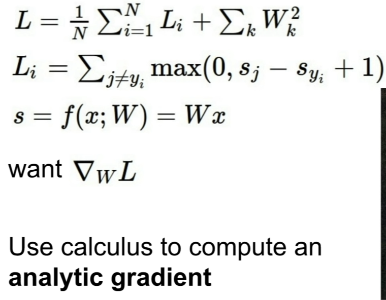
• $\nabla_WL$은 $W$를 변화시켰을 때 $L$이 얼마나 변하는지에 대한 값임
  • $L$을 $W$에 대해 편미분한 것

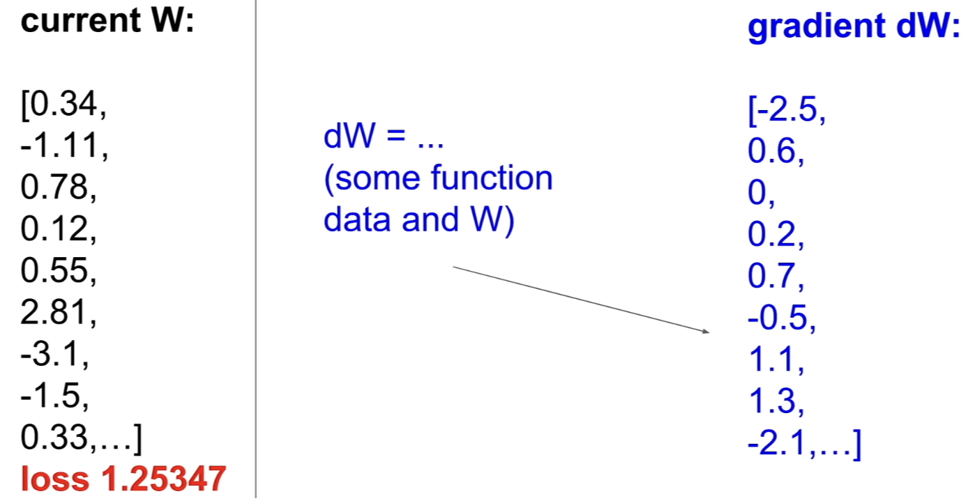
• write the expression for our loss and an expression for what this gradient should be (using calculus)
  • more efficient that trying to compute it analytically via finite differences
• figure ahead of time what the analytic expression for the gradient is, and go directly from the $W$ and compute the $dW$ or the gradient in one step

Summary so far

• Numerical gradient - approximate, simple, slow, easy to write
  • but a very useful debugging tool
• Analytic gradient - exact, fast, error-prone
• In practice, always use analytic gradient, but check implementation with numerical gradient = gradient check

Gradient Descent

• once we know how to compute the gradient, it leads us to a simple algorithm but heart of how we train these very biggest, complex algorithms

# Vanilla Gradient Descent

while True:
	weights_grad = evaluate_gradient(loss_fun, data, weights)
    weights += - step_size * weights_grad  # perform parameter update

• after initializing $W$ with some random thing, while True, compute loss in our gradients and update weights in the opposite of the gradient direction

  • why opposite? → gradient is pointing in the direction of greatest increase of the function
    • 미분값이 + 이면 반대로 가야 최솟값에 도달할 수가 있음
    • 반대로 -이면 +로 가야 (반대방향으로) 최솟값에 도달 가능

• step size = learning rate is hyperparameter

  • how far do we step in that direction at every update

• 2D example
  

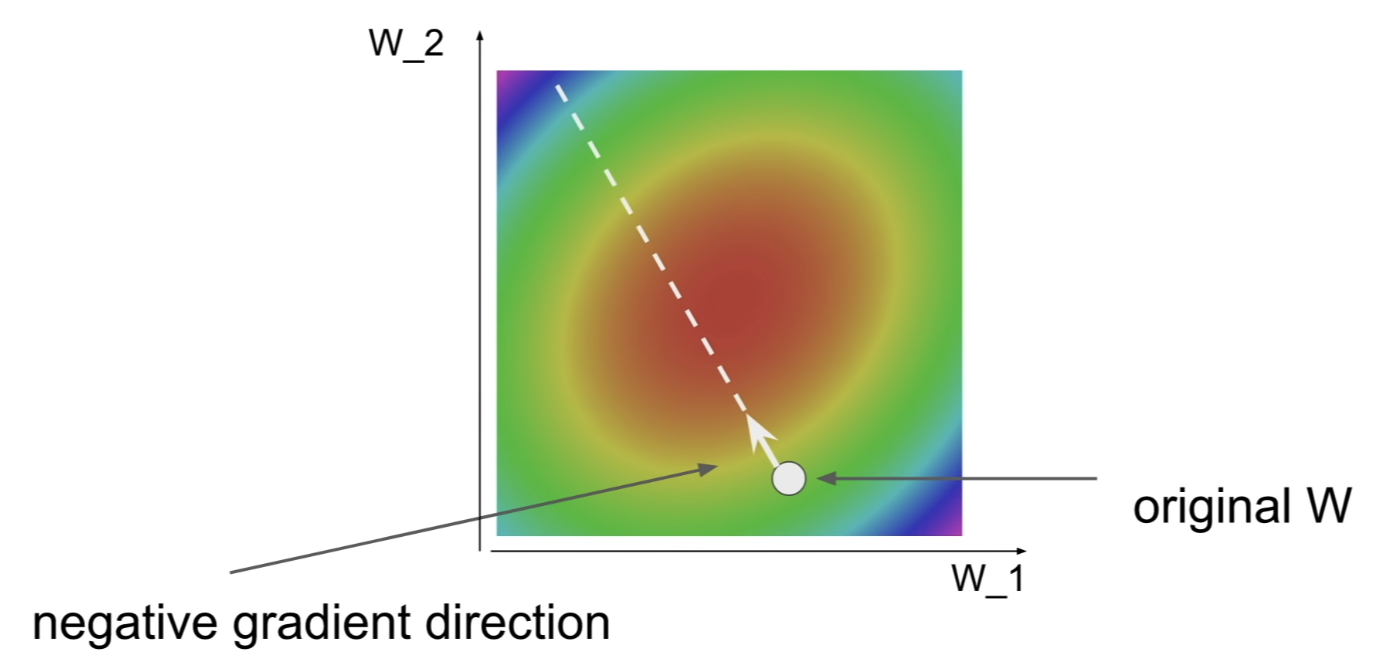
  • bowl = showing loss function (red = low loss = we want to get here)
  • start $W$ at a random point in space, and compute the negative gradient direction, repeat, and hopefully it'll get to the exact minima

Stochastic Gradient Descent (SGD)

• we defined...
  • a loss as computing how bad a classifier is doing at any single training example
  • a full loss as average loss across the entire training set
• $N$(데이터 개수) could be very large in practice
  • ex) image data set → N = 1.3 million
    • computing this loss is very expensive and requires a lot of computing → could be very slow
  • gradient is a linear operator
    • the gradient of the loss is the sum of gradient of the losses for each of the individual terms
  • so, if we want to compute the gradient again, it requires to iterate over the entire training data set, if N = million → very slow
  • In practice, we use SGD
• rather than computing the loss and gradient over the training set, every iteration, we sample some small set of training example called minibatch (32, 64, 128 are common numbers)
  • use minibatch to estimate the full sum, estimate the true gradient
• this is stochastic(확률적)
  • b/c you can view this as Monte Carlo estimate of some expectation of the true value
    • Monte Carlo - 반복된 무작위 추출을 이용하여 함수의 값을 수리적으로 근사하는 알고리즘 (추정하고 싶은 값을 random sampling을 통해 근사하는 것)

# Vanilla Minibatch Gradient Descent
while True:
	data_batch = sample_training_data(data, 256)  # sample 256 examples
    weights_grad = evaluate_gradient(loss_fun, data_batch, weights)
    weights += - step_size * weights_grad  # perform parameter update

• sample some random minibatch of data → evaluate loss and gradient on the minibatch → make an update of the parameter based on the estimate of the gradient

Aside: Image Features

• input raw pixel values into linear classifier = not work so well
  
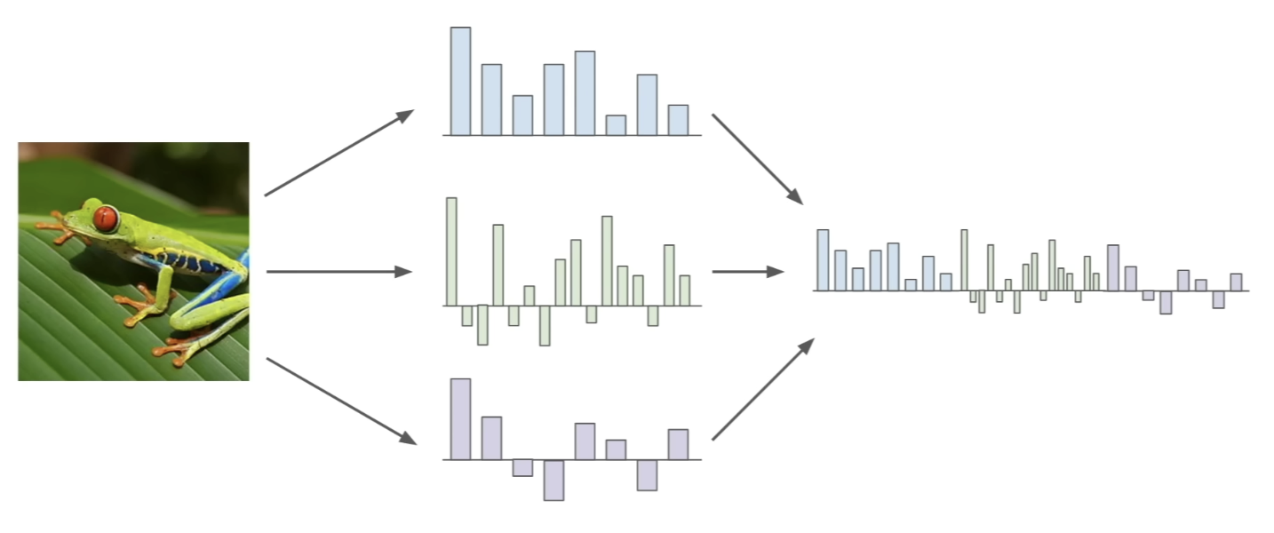
• before the dominance of deep neural network, using 2-stage apporach was common
  • compute various feature representations of input image
  • concatenate these different feature vectors to get feature representation of the image
    • this feature representation of the image is the input to a linear classifier, rather than the raw pixel values

Motivation

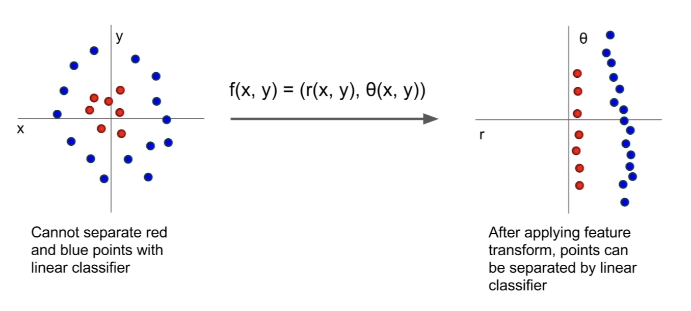
• training data set on the left
  • no way that we can draw a linear decision boundary to separate blue and red points
• but if we use a clever feature transform (in this case transforming to polar coordinates)
  • after doing the feature trasnform, this complex data might become linearly separable
  • and could be classified by a linear classifier
• now, figure out what the right feature transform that is computing the right quantities for the problem is
  • ex) images - converting pixels to polar coordinates doesn't make sense, but you can try to write down feature representations of images that might make sense and might do better than putting raw pixels in the classifier

Example: Color Histogram

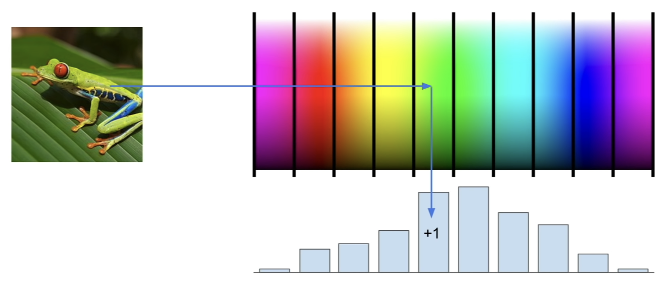
• take hue color spectrum and divide into buckets
• for every pixel, map it into one of the color buckets and count how many pixels fall into each buckets
• this is an example of a simple feature vector

Example: Histogram of Oriented Gradients (HoG)

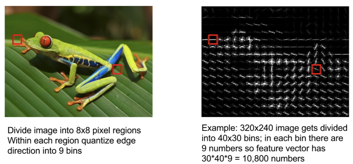
• oriented edges are important in the human visual system (Hubel and Wiesel)
• this histogram tries to capture the same intuition and measure the local orientation of edges on the image
  • divide the image into 8x8 pixel regions
  • within each region, compute what the dominant edge direction is
  • quantize those edge directions into several buckets
  • within each region, compute a histogram over these different edge orientations
• full-feature vector would be bucketed histograms of edge orientations across all the different 8x8 regions

Example: Bag of Words

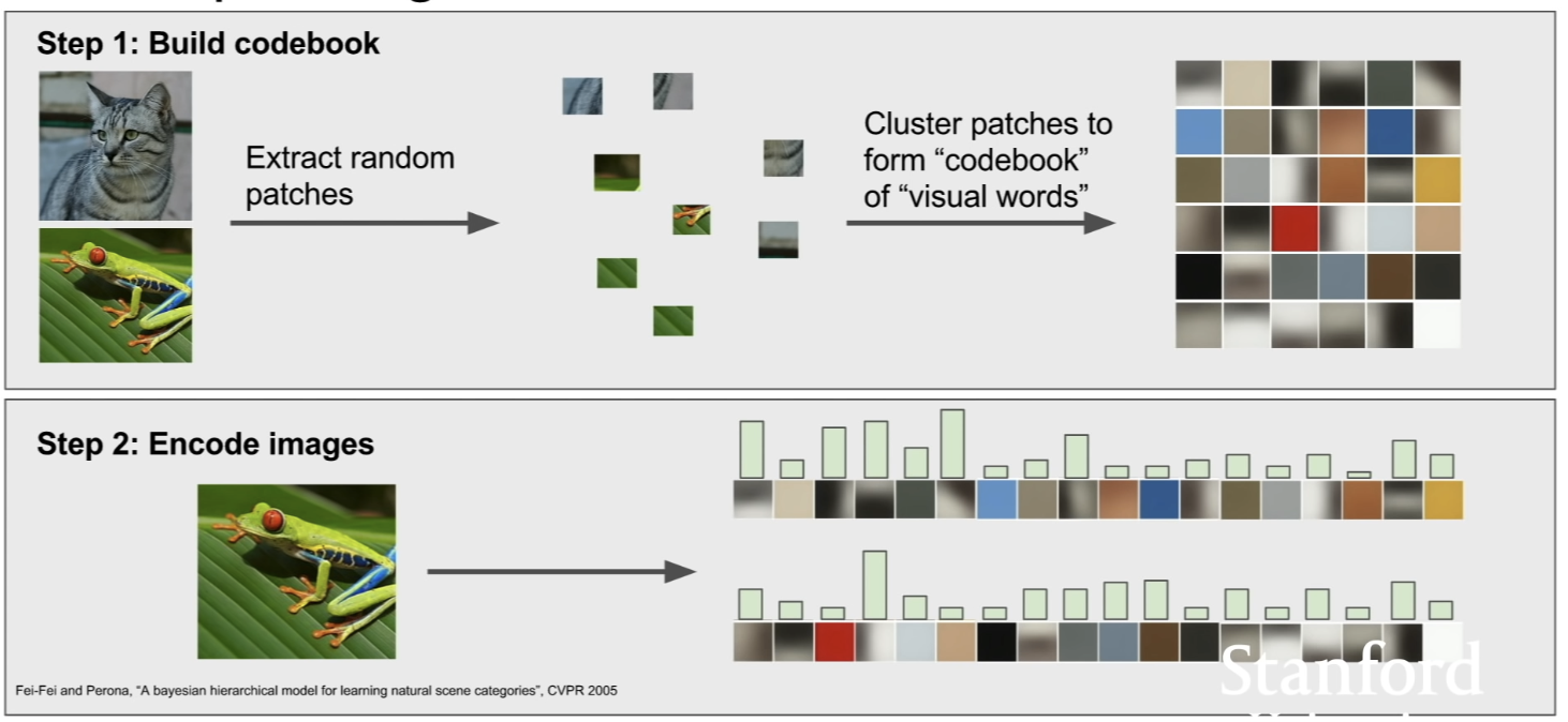
• a way to represent a paragraph might be counting up the occurrences of different words → apply it into images someway
• so, we need to define our own "vocabulary" of visual words → 2-stage approach
  • get a bunch of images, sample a group of tiny random crops from those images
  • cluster them using K-means
    • to come up with different cluster centers that might be representing different types of visual words in the images

Summary (image features vc convnets)

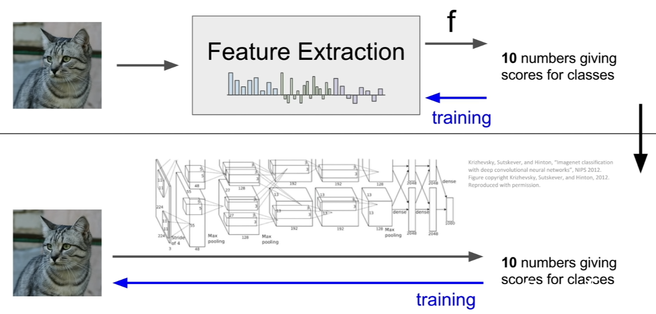
• way that the image classification pipeline might have looked like 5-10 years ago, would be compute the different feature representations of the image(ex. bag of words) → concatenate a whole bunch of feature together, feed this feature extractor down into linear classifier
  ⇒ after extracting the feature, this feature extractor would be a fixed block that would not be updated during training. during training, only linear classifier that's working on top of features would be updated.
• BUT in ConvNets, rather than writing down the feature ahead of time, we're going to learn the features directly from the data
  • train this entire weights for this entire network rather than just the weights of the linear classifier on the top