🔎 Stanford CS231n 강의를 듣고 기록용도로 정리하는 게시글입니다.
- how to compute analytic gradient for arbitrarily complex functions using a framework called computational graphs
Computational graph
- With computational graph, we can represent any functions
- nodes: steps of computation we go through
-
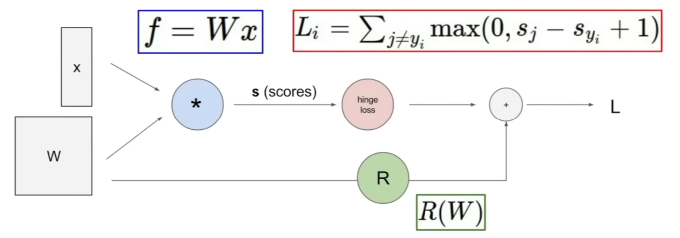
A computational graph for a linear classifier
- input: (data), (parameters)
- * node: multiplication of and
- node: computes data loss term
- regularization node: computes regularization term
- : sum of regularization term and the data term
-
Advantage: we can use backpropagation
- backpropagation: using the chain rule in order to compute the gradient of every variable in the computational graph
- useful for a complex function
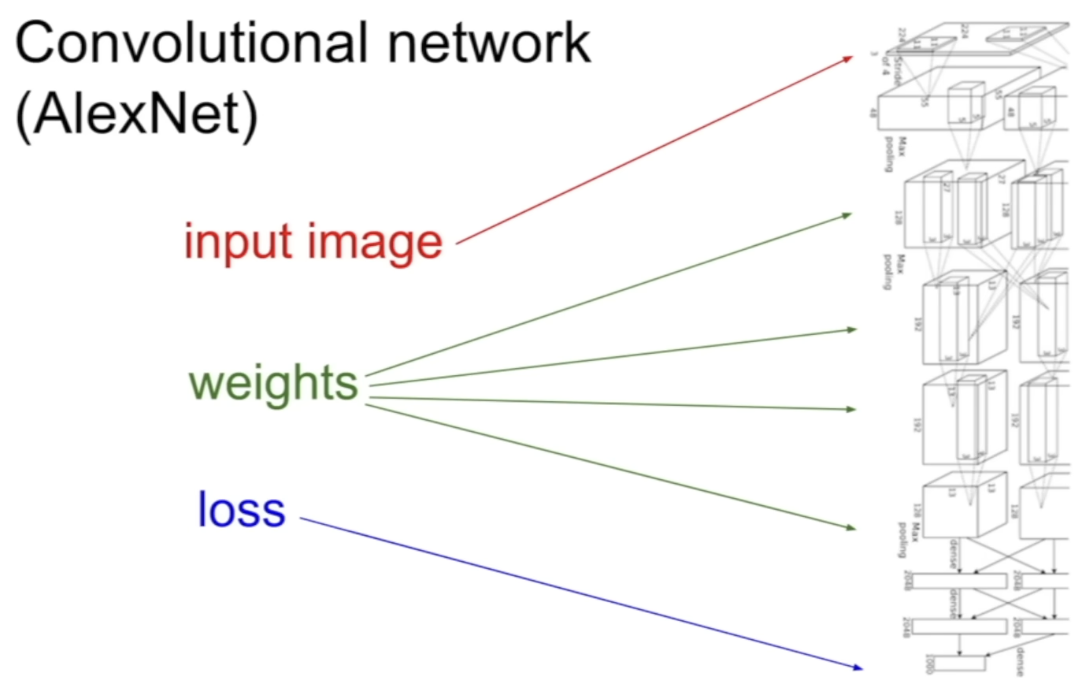
- input image at the top, loss at the bottom
- input has to go through many layers
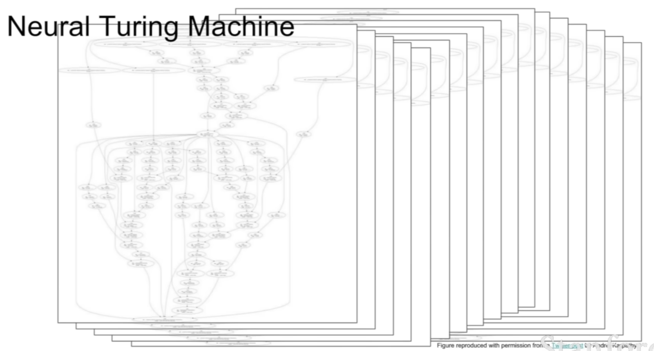
- neural turing machine - graph is insane, very impractical if you want to compute the gradients for any of these intermediate variables
Backpropagation
A simple example
- Goal: find the gradients of the output of the function with respect to any of the variables
- Take the function , represent it using a computational graph
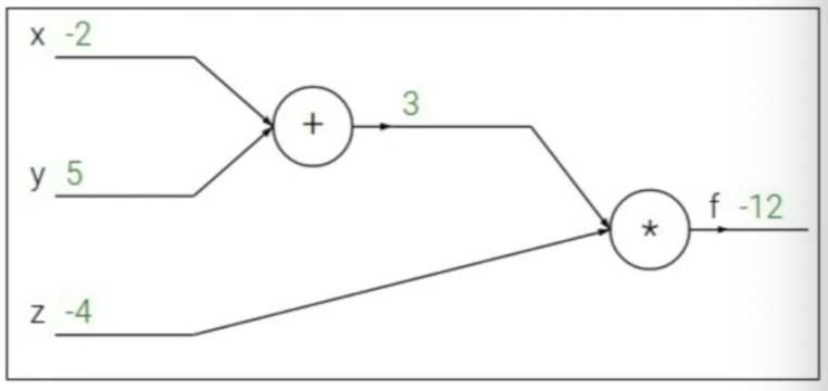
- Forward pass; given the value(), fill these all in the graph and compute an intermediate value()
- Assign a name to every intermediate value
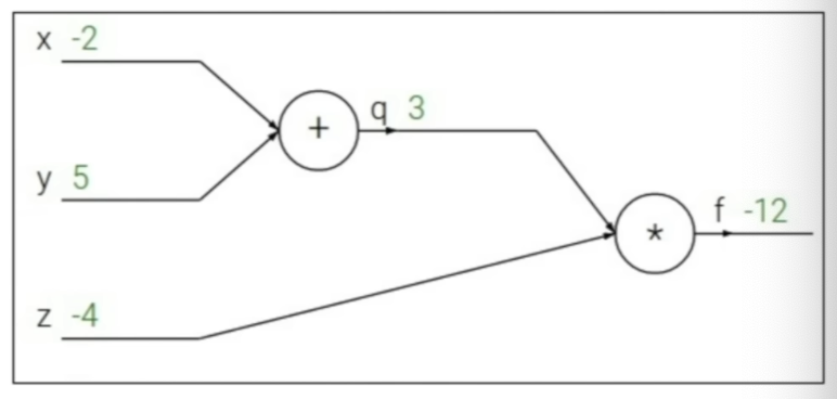
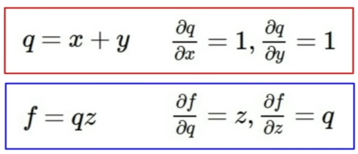
- gradients of with respect to and = 1 (b/c of the addition)
- gradients of with respect to and are and (b/c of the multiplaction rule - 를 에 대해 미분한 결과는 계수였던 임)
- What we want:
- Backprop is a recursive application of chain rule, starting at the back, work our way backwards and compute all the gradients along the way
- Start at the back
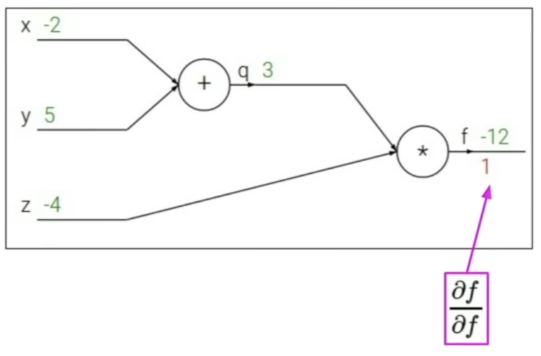
- gradient of the output with respect to the last variable(=f) = 1
- Now, we want the gradient with respect to .
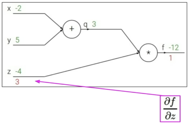
- we know:
- We want the gradient with respect to
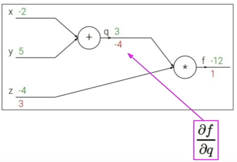
- want , which is
- Now, we want to compute , but is not connected directly to . BUT connected through intermediate node () ⇒ leverage chain rule
- Gradient with respect to , so we want , follow the same procedure as step4
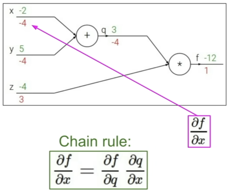
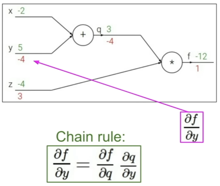
-
Each node of the computational graph is only aware of its immediate surroundings.
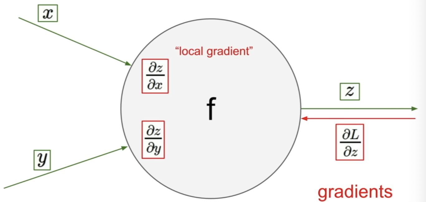
- Local inputs and outputs that are directly connected to this node
- In this case, local inputs = and , output =
- And for each node, we can compute the local gradient(gradient of with respect to and )
- These operations in each node is simple
-
Backprop
- Each node has upstream gradients with respect to the immediate output of the node coming back
- So when we reached this node, we've already computed the gradient of our final loss with respect to
- Now, we want to find the gradients with respect to just before the node = to the values of and
- Here, use the chain rule = take the upstream gradient coming down and multiply it with the local gradient in order to get the gradient with respect to the input
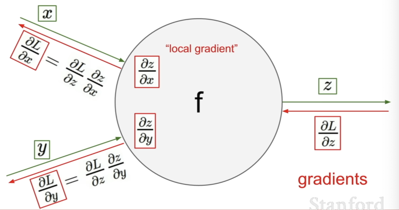
- Here, use the chain rule = take the upstream gradient coming down and multiply it with the local gradient in order to get the gradient with respect to the input
-
결론: At each node, compute the local gradient and keep track of it. During backprop, as we receive numerical values of gradients coming from upstream, multiply it by local gradient, send it back to the next nodes going backwards.
More complex example
- Draw a computational graph
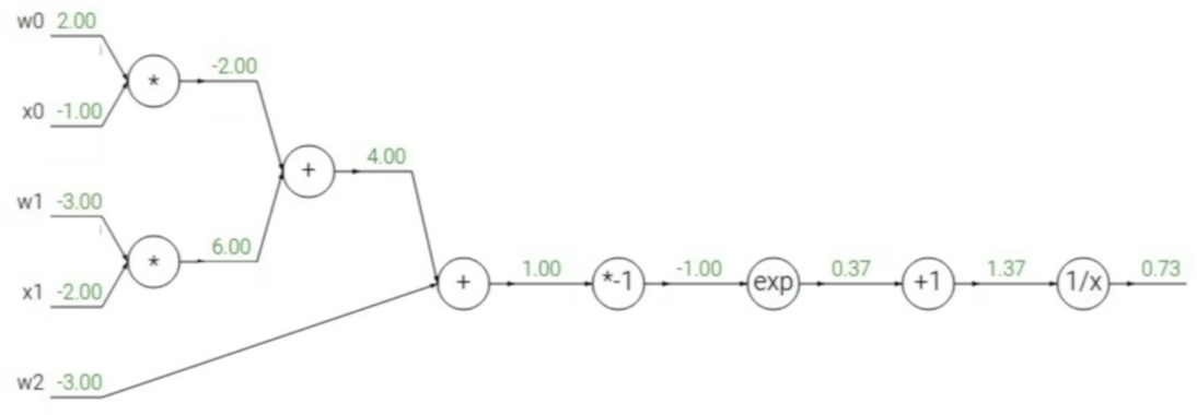
- Start backprop, at the end.
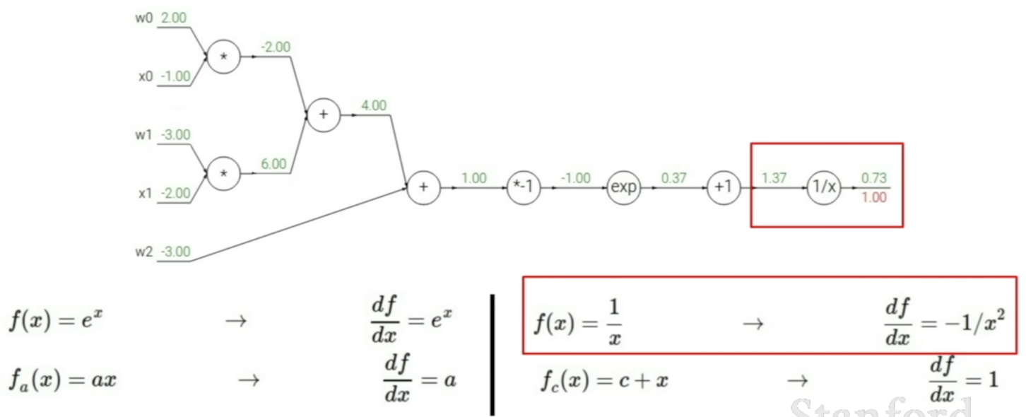
- Gradient with respect to the input just before
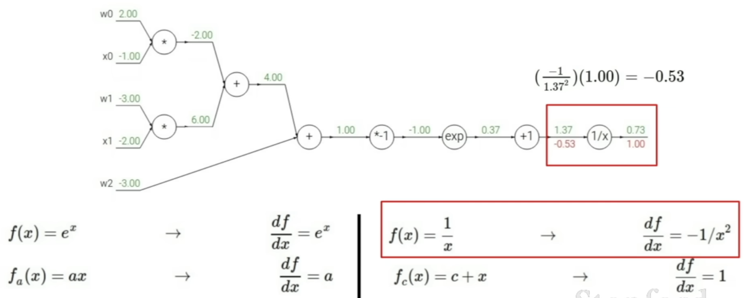
- node's local gradient =
- take , plug in the value of that was the input of this node = 1.37 → -0.53
- Current node = node
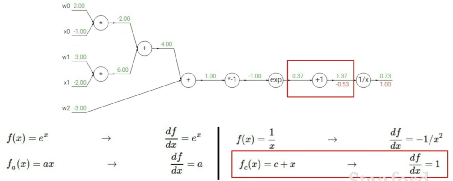
- -0.53(=upstream gradient) * 1 (=local gradient) = -0.53
- current node = node
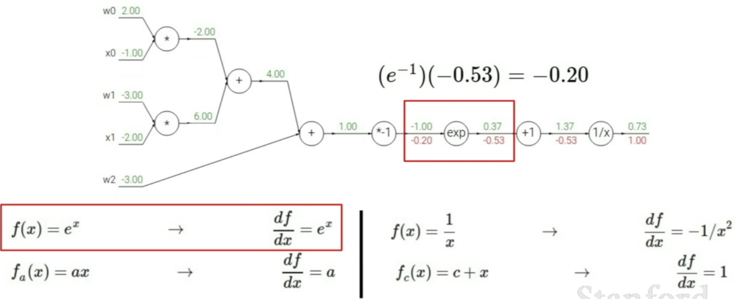
- upstream gradient = -0.53
- local gradient =
- gradient =
- current node = node
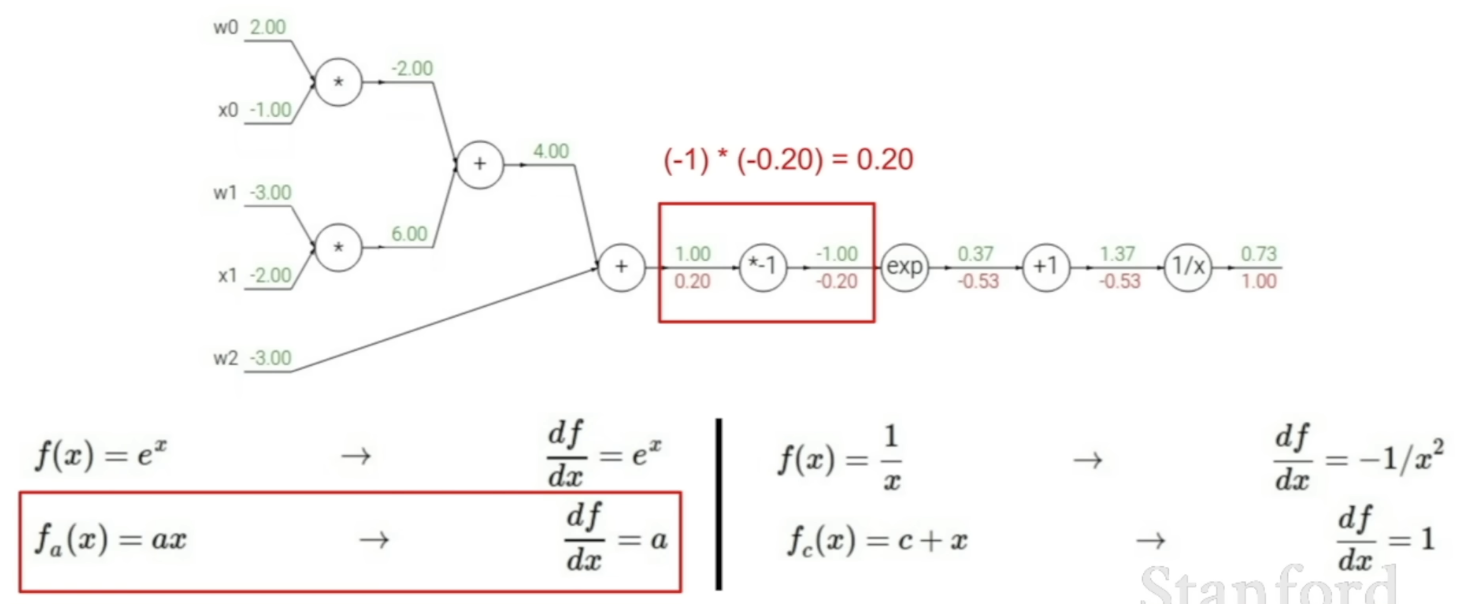
- upstream gradient = -0.2
- local gradient = -1
- gradient = -0.2 * -1 = 0.2
- current node = node
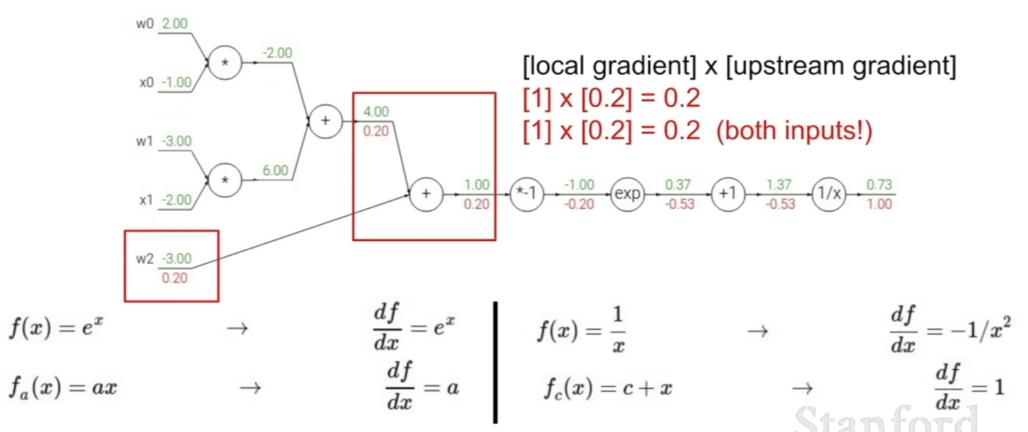
- Here, two branches are connected to this node
⇒ We have to compute the gradient with respect to each of these branches - upstream gradient = 0.2
- the gradient with respect to each of the inputs of an addition node = 1, so top branch = , bottom branch =
- Here, two branches are connected to this node
- current node = node (reached )
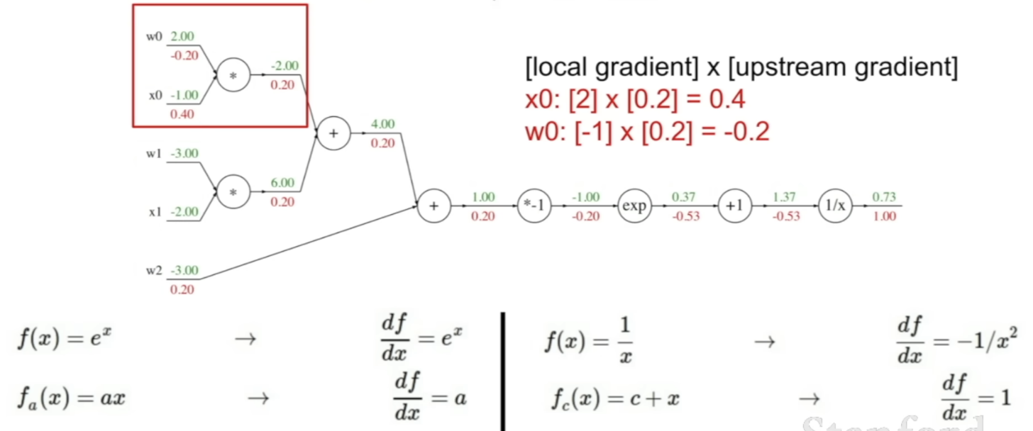
- upstream gradient = 0.2
- gradient with respect to = 2 * 0.2 = 0.4
- gradient with respect to = -1 * 0.2 = -0.2
Why do we use backprop
- Why is this simpler than computing, deriving the analytic gradient?
- All we ever dealt with was expressions for local gradients.
- Once we had expressions for local gradients, all we did was to plug in the values for each of these we had and use the chain rule to numerically multiply this all the way backwards and get the gradients with resepct to all of the variables.
Sigmoid function
- When creating computational graphs, we can define the nodes at any granularity(입상,입도) that we want to.
- Until now, we broke it down into the absolute simplest that we could (ex. addition, multiplication)
- But in practice, we can group some of these nodes into more complex nodes as long as we're able to write the local gradient for that node
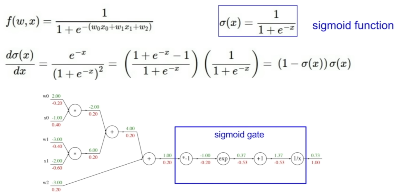
- We can compute the gradient for sigmoid function, which can get us a nice expression at the end ()
- all this is a trade-off between how much math you have to do in order to get a more, concise, simpler graph vs. how simple you want each of the gradients to be.
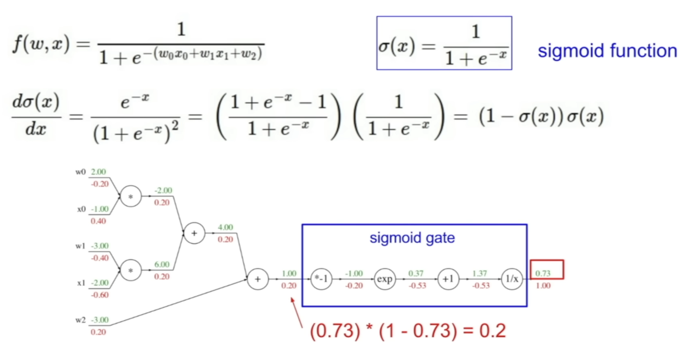
- input to the sigmoid gate = 1.00
- output of the sigmoid gate = 0.73
- Now, we want to take the gradient, treat this gate as one node → use the local gradient derived above
- (=output), so, =
local gradient - upstream gradient = 1
- multiply them → 0.2 * 1 = 0.2
- (=output), so, =
Patterns in backward flow
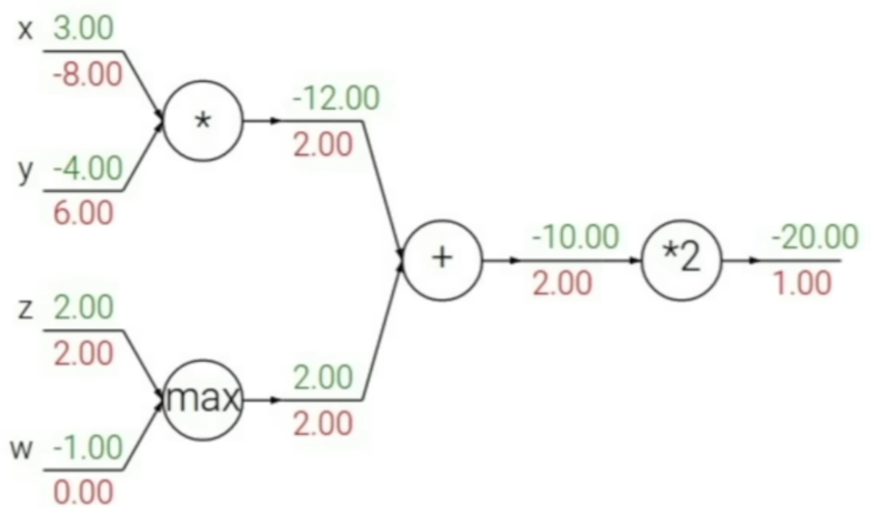
ADD gate: gradient distributor
- When we pass through ADD gate, the upstream gradient is passed on to the input branches.
MAX gate: gradient router
- input: and
- operation: take the max, which is 2, pass it down into the remainder of the computational graph
- upstream gradient = 2, local gradient of
- One of these will get the full value of the gradient that's passed back and the other one will have a gradient of 0
MAX gate will take the gradient and route it to one of the branches
MUL gate: gradient switcher
- MUL gate takes the upstream gradient and scale it by the value of the other branch.
Branches: where gradients are added at
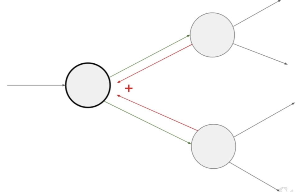
- When we have a place where one node is connected to multiple nodes, gradients add up at this node.
- Take the value of upstream gradients, add these together to get the total upstream gradient that's flowing back into this node.
- If we change this node a little bit, it's going to affect both of these connected nodes when doing forward pass.
- When backprop, both of gradients coming back are going to affect this node.
Gradients for vectorized code
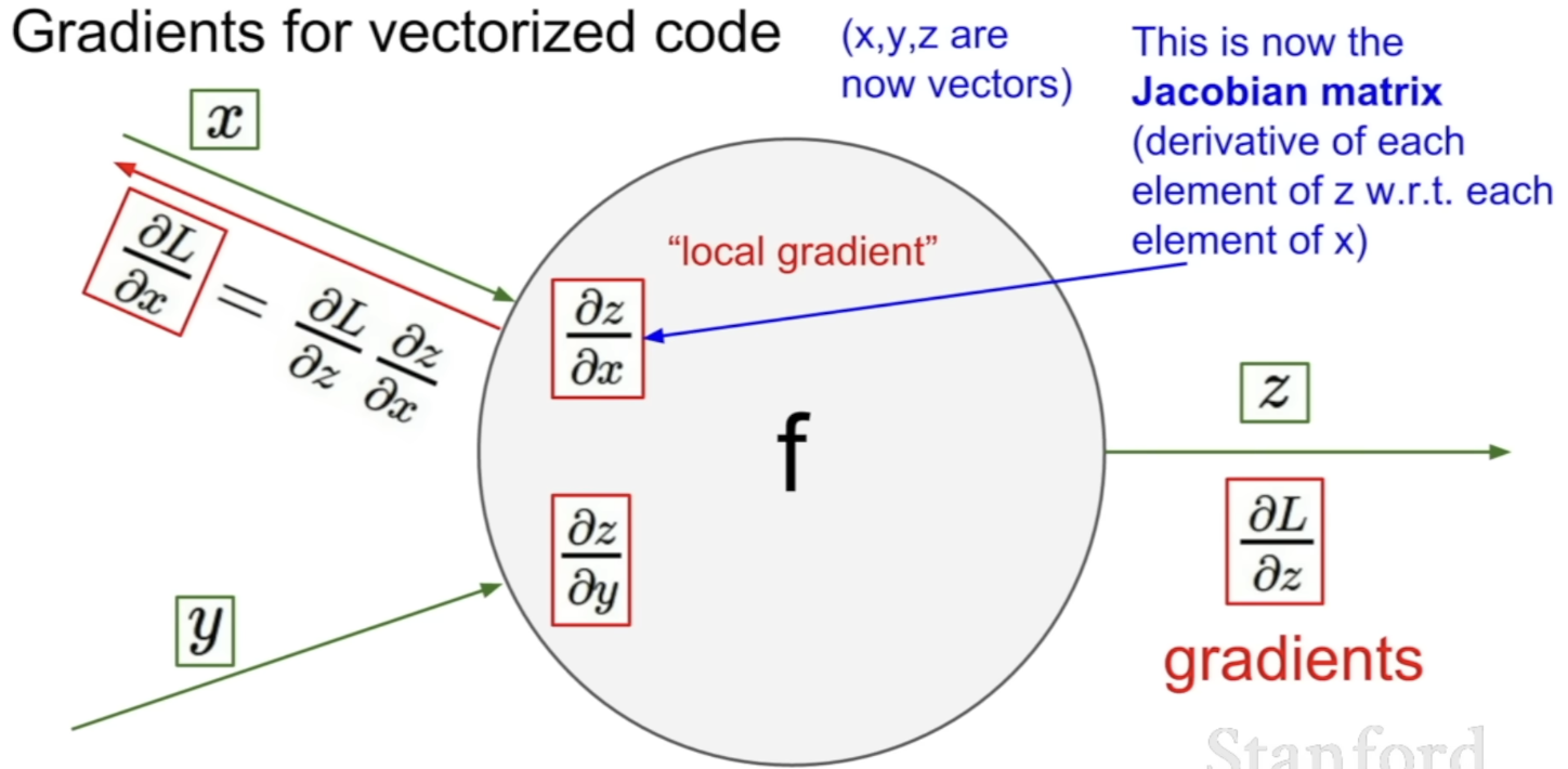
- What happens when we have vectors?
- The entire flow stays exactly the same, but the only difference is that now our gradients are going to be Jacobian matrices
- matrices containing the derivative of each element of, for example z, with respect to each element of x
- Each row is a matrix of partial derivatives of each dimension of the output with respect to each dimension of the input.
Vectorized operations
- input: vector (4096-dimension input vector)
- node: element-wise maximum
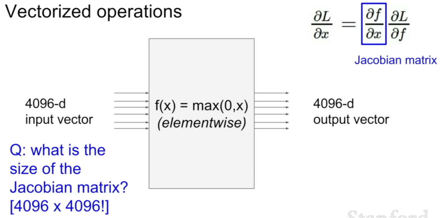
- What is the size of the Jacobian matrix?
- Jacobian matrix will be 4096 x 4096 → very large
- In practice, this is going to be even larger, b/c we're going to work with many batches of 100 inputs at the same time, and put all of them at the same time → very impractical
- But in practice, we don't need to compute this hugh jacobian most of the time, why?
- What does the Jacobian matrix look like? (?)
- Which dimension of the input affects which dimensions of the output?
- What sort of structure can we see in our Jacobian matrix?
⇒ Diagonal matrix- ex) in first dimension, each element of the input, only affects that corresponding element in the output
- in practice, we don't have to write out the entire Jacobian, but just know the effect of x on the output, and use these values and fill it in as we're computing gradient
Example
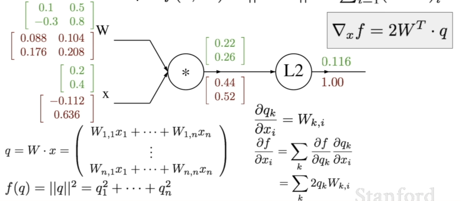
- is n-dimensional, is n x n
- Start by computational graph
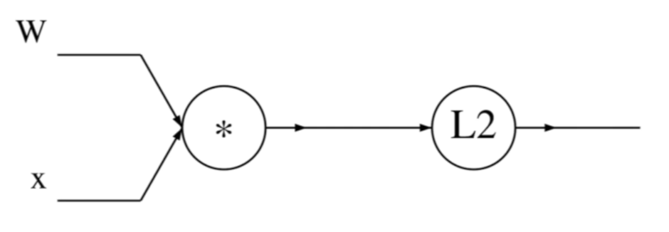
- Set intermediate nodes
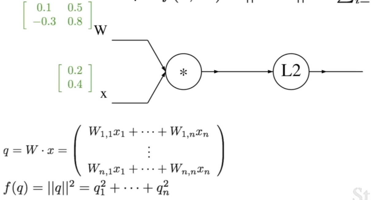
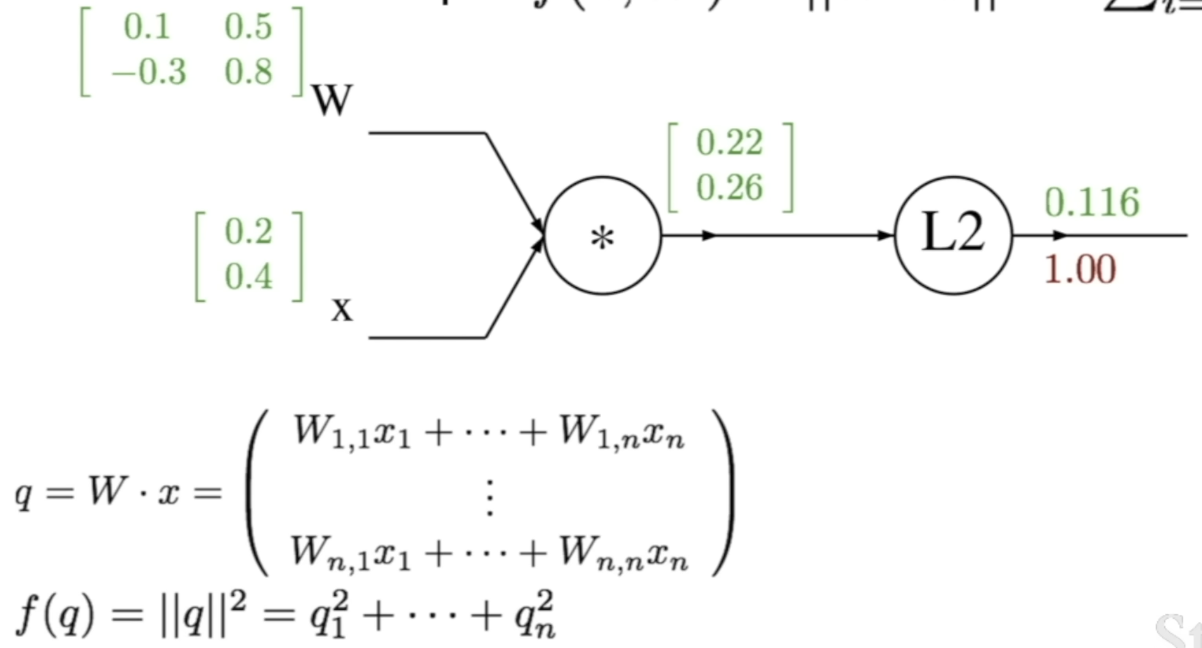
- Say that is 2x2 matrix, is 2-dimensional vector.
- = intermediate node after the multiplication
- Gradient with respect to the output = 1
- Find the gradient with respect to , which is intermediate variable before the
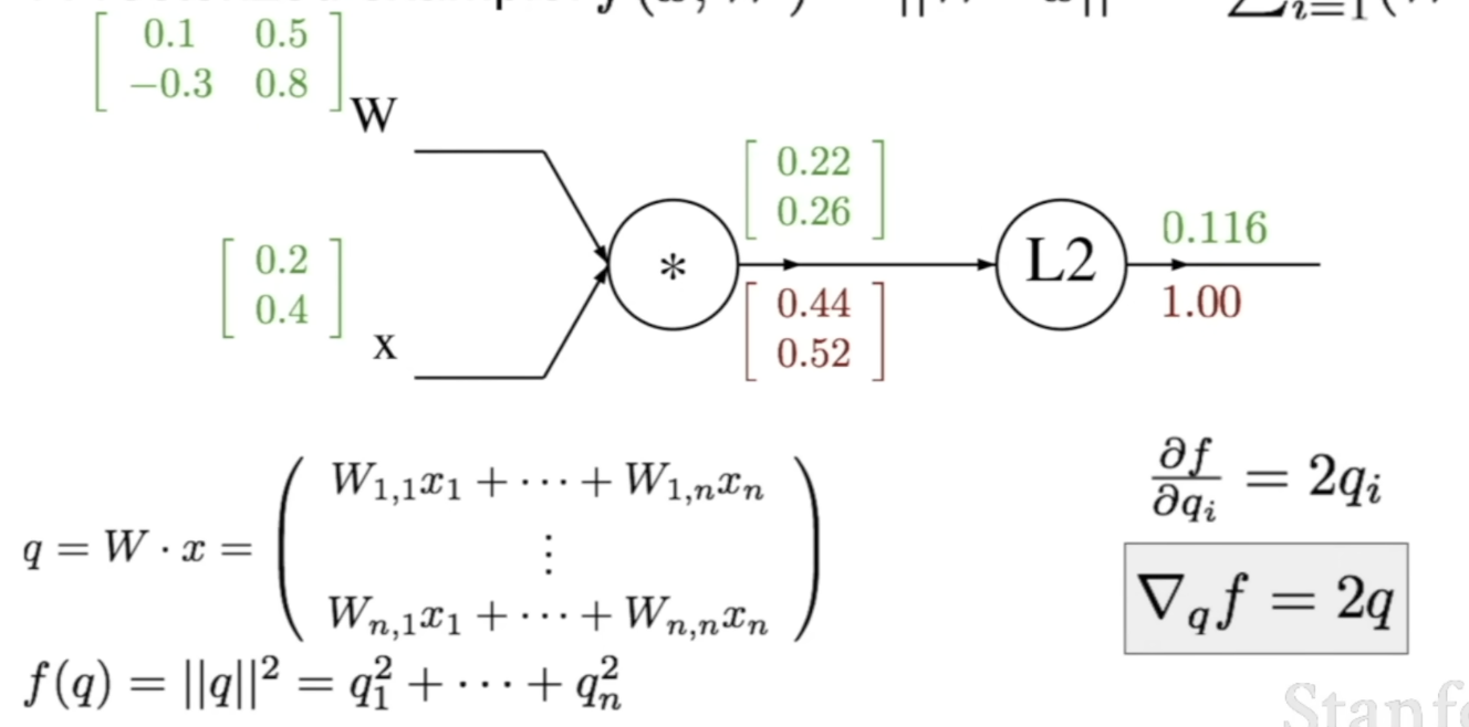
- is 2-d vector, and we want to find how each element of affects the final value of
- Gradient of with respect to a specific is (제곱을 미분)
- So, take and scale it by 2 and we get
- So, the gradient of the vector is always the same size as the original vector, and each element of this gradient means how much of this particualr element affects our final output of the function.
- Find the gradient with respect to .
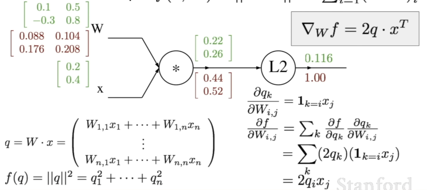
- compute local gradient of with respect to
- look at things element-wisely
- see what the effects of each element of is to each element of
- ex) gradient of the first element of () with respect to =
- more generally,
- compute local gradient of with respect to
- Important thing is to always check that the gradient with respect to a variable has the same shape as the variable.
- Find the gradient with respect to
Modularized implementation: foward, backward API
-
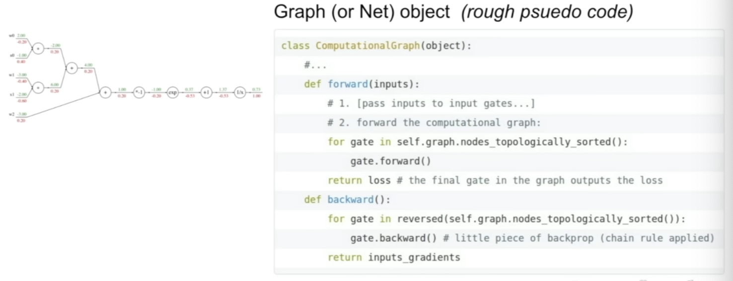
In our computational graph, we looked at each node locally and computed the local gradients and chained them with upstream gradients coming down.
-
You can think of this as forward and backward api.
-
Forward pass: implement a function computing the output of this node -
backward pass: compute the gradient -
implement this in code, exactly the same way
-
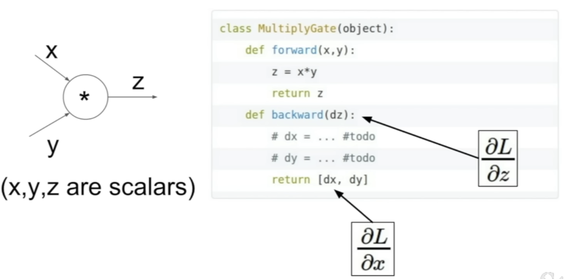
implementation for MUL gate
- implementation the
forward pass: getsxandyas inputs, returns valuez- important: we need to cache the values of the forward pass b/c we end up using them in the backward pass a lot of the time
backward pass: getdzas input(=upstream gradient), output the gradients on the input'sxandyto pass down
- implementation the
Example: Caffe layers
- Caffe: a famous deep learning framework
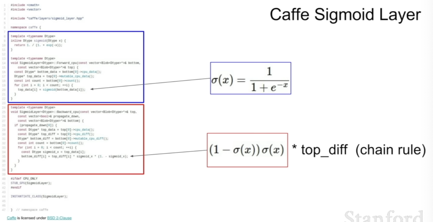
- There's a forward pass which computes the sigmoid expression
- Backward pass: takes
top_diffas input(upstream gradient) and multiply it by local gradient that we computed.
Summary so far
- Neural nets will be very large: impractical to write down gradient formula by hand for all parameters
- in order to get these gradients, we use Backpropagation
- Backpropagation = recursive application of the chain rule along a computational graph to compute the gradients of all inputs/parameters/intermediates
- Implementations maintain a graph structure, where the nodes implement the forward() / backward() API
- forward: compute result of an operation and save any intermediates needed for gradient computation in memory
- backward: apply the chain rule to compute the gradient of loss function with respect to the inputs
Neural networks
Without the brain stuff
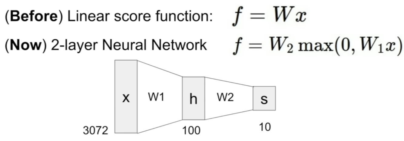
-
Instead of using a single linear transformation, if we want a neural network, we can stack two of these together(simple form) ⇒ get a 2-layer network
-
Neural networks are a class of functions where we have a simpler functions that are stacked on top of each other → stack them in a hierarchical way in order to make up a more complex non-linear function
-
They have multiple stages of hierarchical computations.
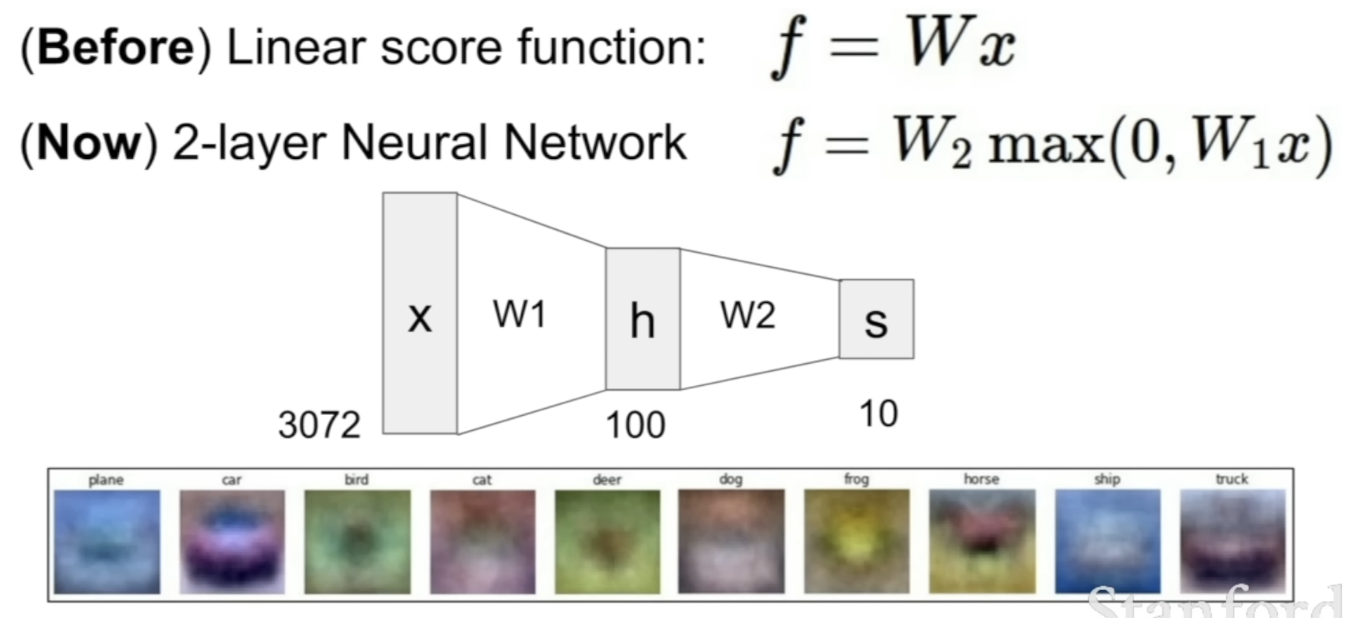
-
Weight matrix was something like a template
- A template that expresses what we're looking for in the input for a specific class
- But the problem was that there's only 1 template per class; we might have a yellow car,.. etc rather than red car
-
Now, can still be those kinds of templates, but each of this intermediate variable , has scores for these templates, and we have another layer on top that combines these together.
- ex) is like a weighted sum of all of the templates(ex. left-facing horse, right-facing horse, etc)
Analogy between neuron and computational graph
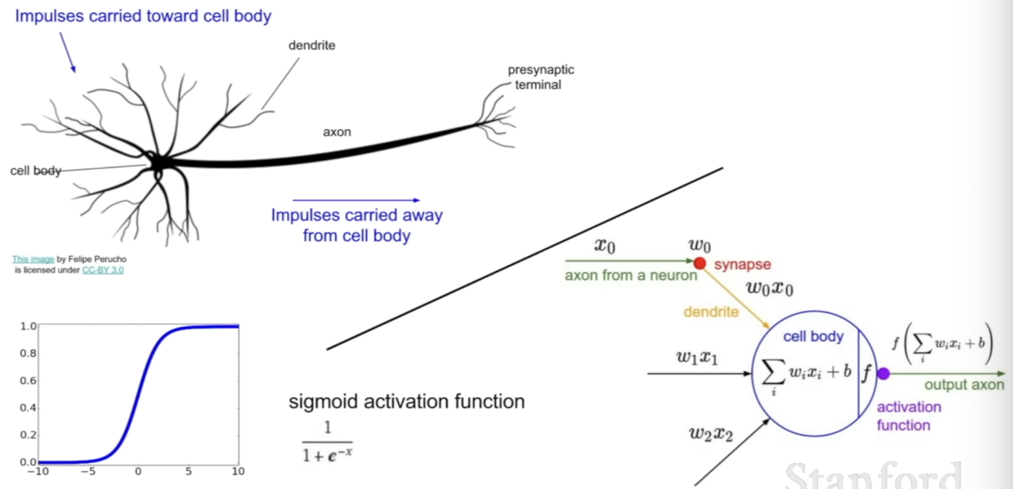
-
Neuron has impluses carried towards each neuron.
- A lot of neurons are connected together.
- Each neuron has dendrites, that receive impulses.
-
Cell body integrates signals that are coming in → pass on → carries away to downsteam neurons that are connected to, and carries this away through axons
-
With each computational node, you can see it in a similar way
- Nodes are connected to each other in the computational graph
- inputs or signals, , coming into a neuron
- all of these are combined, integrated together using, weights .
- we have an activation function on the top and get the value of this output and pass it down to the connecting neurons
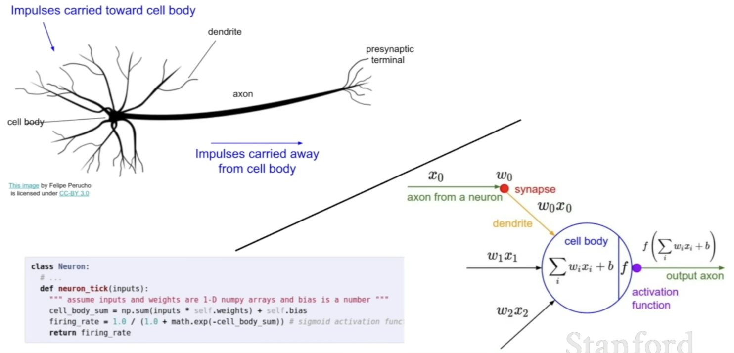
- Also, non-linearities like sigmoid function represent something like firing or spiking rate of neurons.
- And neurons transmit signals to connecting neurons using discrete spikes.
- If they're spiking fast, there's a strong signal that's passed later on.
- We can think of this value after our activation function as this firing rate that we're going to pass on.
Be careful with brain analogies
- In practice, biological neurons are way more complex than this.
- Biological neurons
- many different types
- dendrites can perform complex non-linear computations
- synapses are not a single weight but a complex non-linear dynamical system
- rate code(idea of interpreting our activation function as rate code or firing rate) may not be adequate
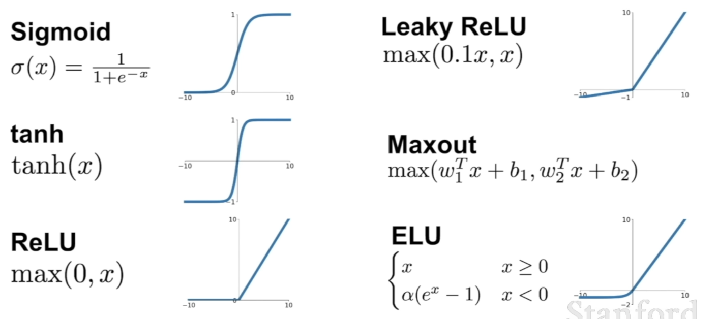
Activation functions
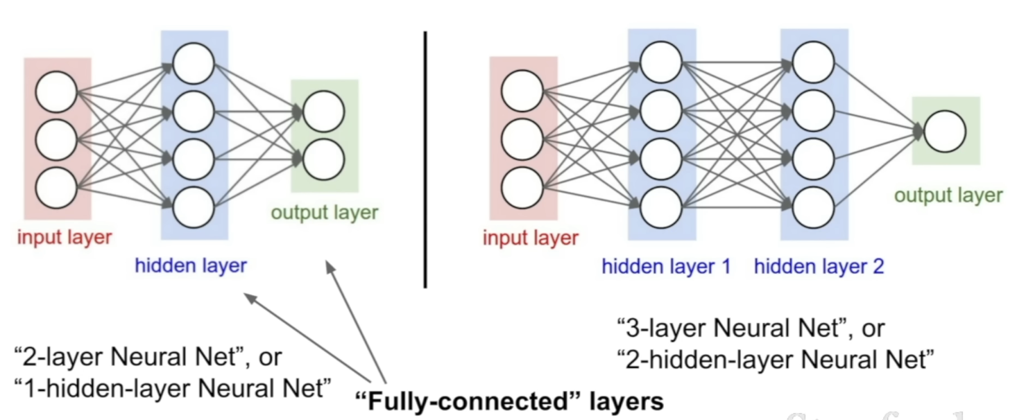
Neural networks: Architectures
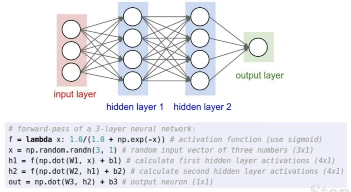
Example feed-forward computation of a neural network
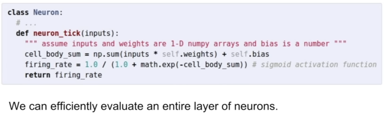
- When doing forward pass through a neural network, each of the nodes in this network is doing the operation of the neuron that was showed earlier.
- Think of each hidden layer as a whole vector, a set of these neurons.
- By writing it with matrix multiplies to compute neuron values, it's a way to efficiently evaluate entire layers of neurons.
- ex) 1 matrix multiply → output value of layer of 10 neurons
Summary
- We arrange neurons into fully-connected layers
- The abstraction of a layer has the nice property that it allows us to use efficient vectorized code (e.g. matrix multiplies)
- Neural networks are not really neural
- it's a loose analogy
- Next time: Convolutional Neural Networks
