🔎 Stanford CS231n 강의를 듣고 기록용도로 정리하는 게시글입니다.
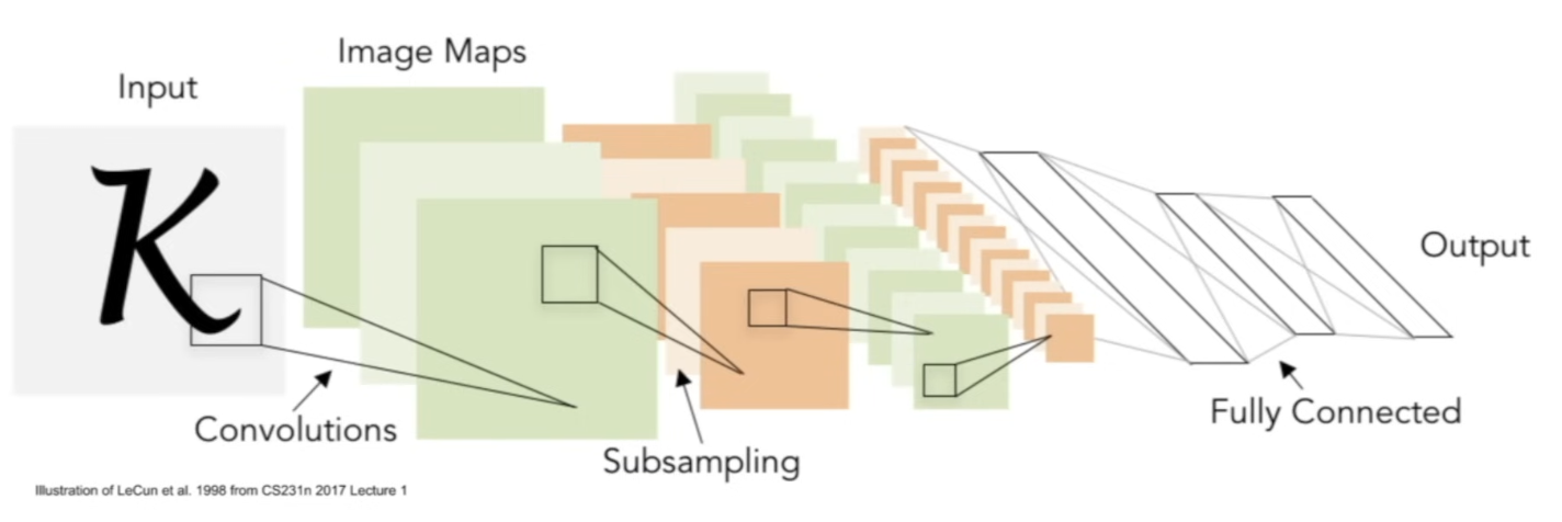
- convolutional layers - maintain spatial structures
History
- 1957, MARK I Perceptron machine
- first implementation of the perceptron algorithm
- similar idea of getting score fucntions, using
- BUT outputs are either 1 or 0 and update rules look similar to backprop but no principled backprop technique yet
- 1960, Widrow and Hoff
- able to stack linear layers into multilayer perceptron networks
- BUT still didn't have backprop or principled way to train this
- 1986, Rumelhart
- backprop was introduced
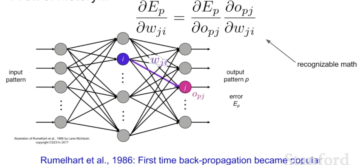
- principled way to train network architectures
- backprop was introduced
- 2006, Hinton and Salakhutdinov
- still not able to scale very large neural networks, so there was a period where nothing new was happening
- started being reinvigorated
- showed that we could train a deep neural network effectively, but not a modern way
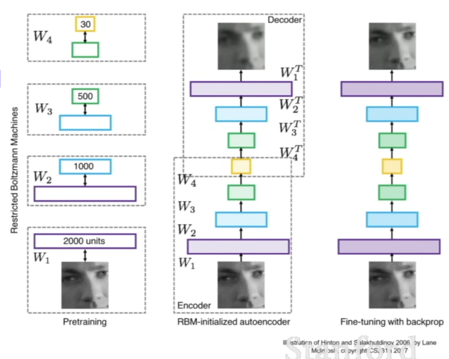
- has a pre-training stage
- where you model each hidden layer, and get initialized weights by training each layers iteratively
- use the hidden layers to initialize full neural network, and do backprop and fine tuning
- first strong results, 2012
- using for speech recognition (hinton's lab)
- image recognition, introduced the first ConvNet, able to reduce the error on image classifier benchmark
What gave rise to CNN?
- Hubel & Wiesel
- topographical mapping in the cortex
- nearby cells in cortext represent nearby regions in the visual field
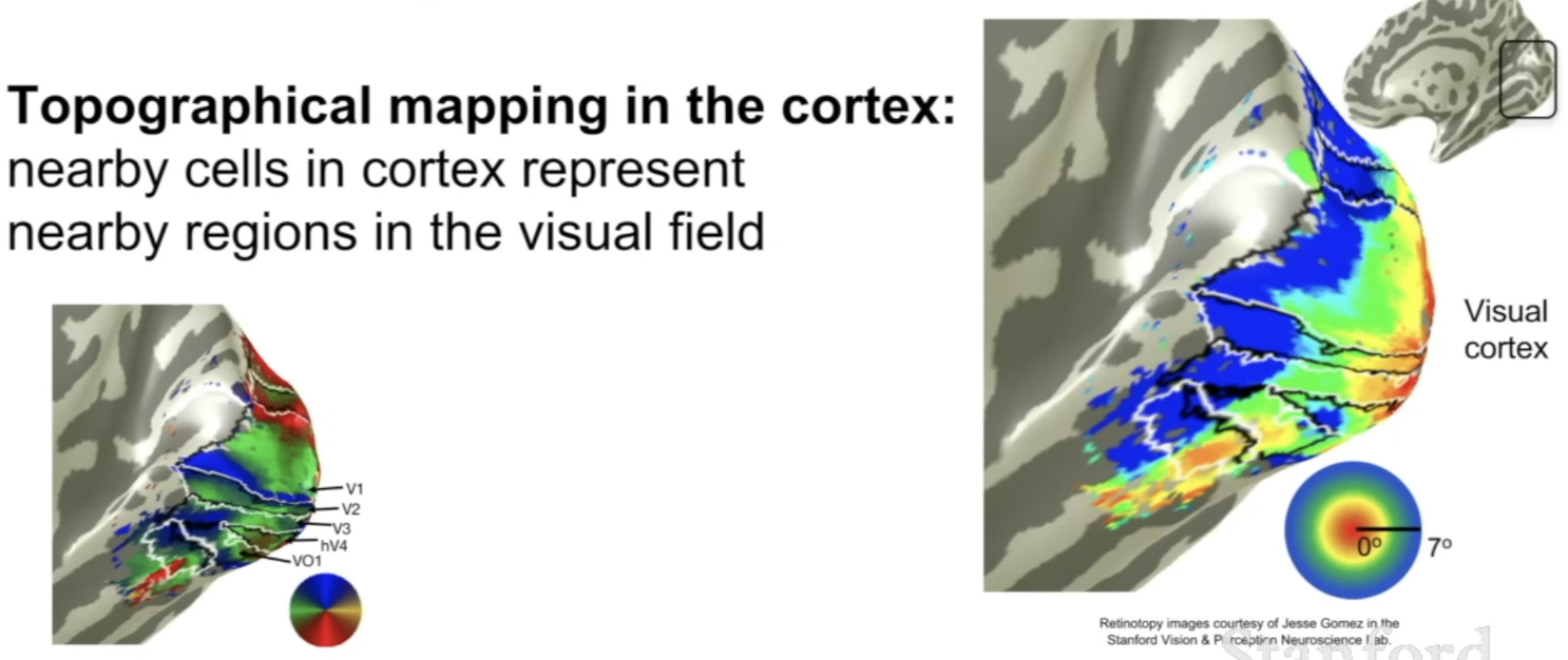
- nearby cells in cortext represent nearby regions in the visual field
- discovered that neurons have hierarchical organization
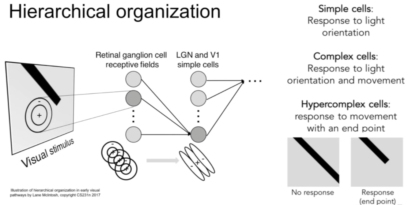
- increasing complexity
- topographical mapping in the cortex
- Neurocognitron, 1980
- first example of a network architecture that has the idea of simple and complex cells above
- simple cells have modifiable parameters, complex cells performed pooling so that it was invariant to different minor modifications from simple cells
- Gradient-based Learning applied to document recognition
- did pretty good on zip code recognition (digit codes)
- ImageNet Classification with Deep Convolutional Neural Networks
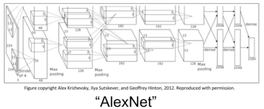
- the modern incarnation of convolutional neural networks = Alexnet
- Now, ConvNets everywhere
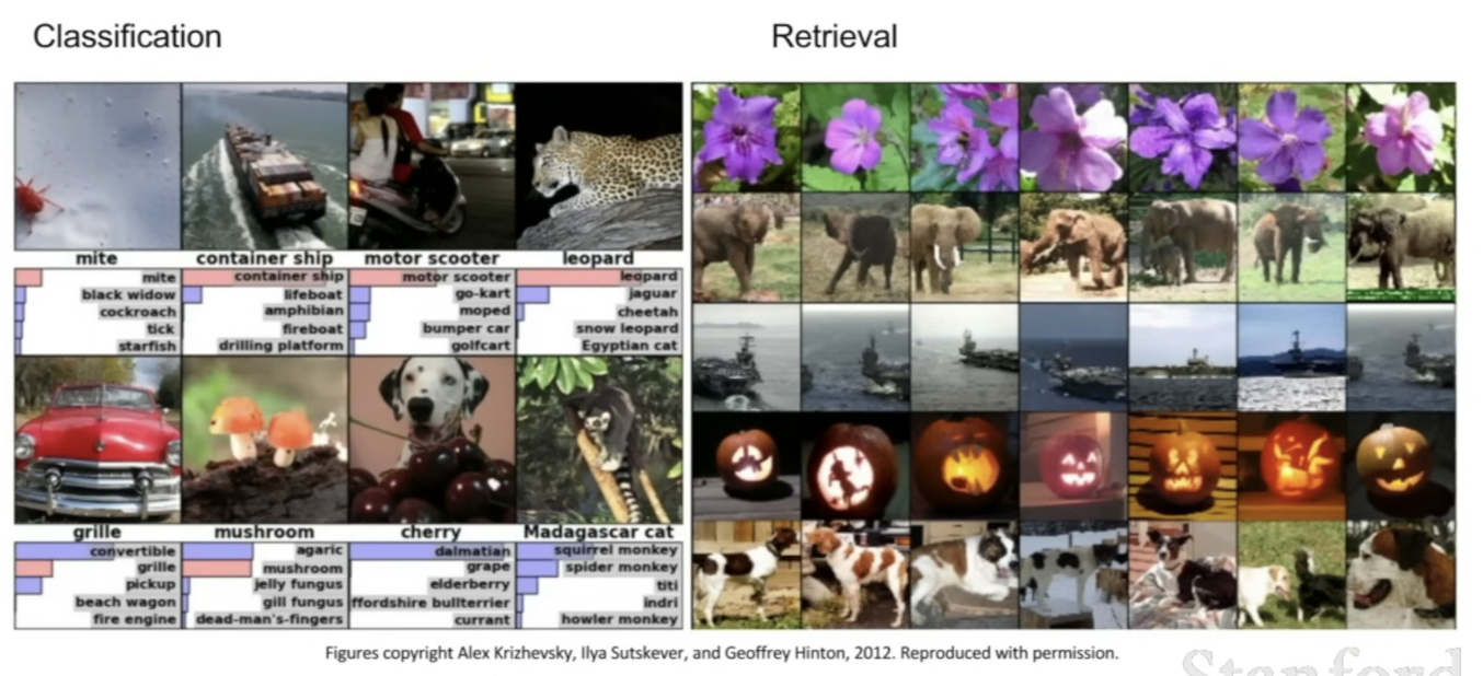
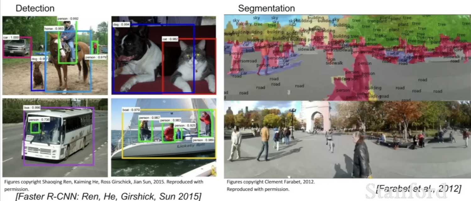
- powered by GPU
- able to do parallel processing and efficiently train and run ConvNets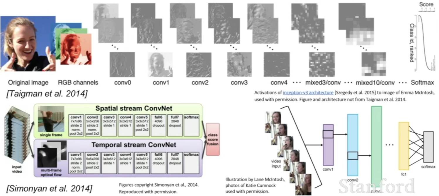
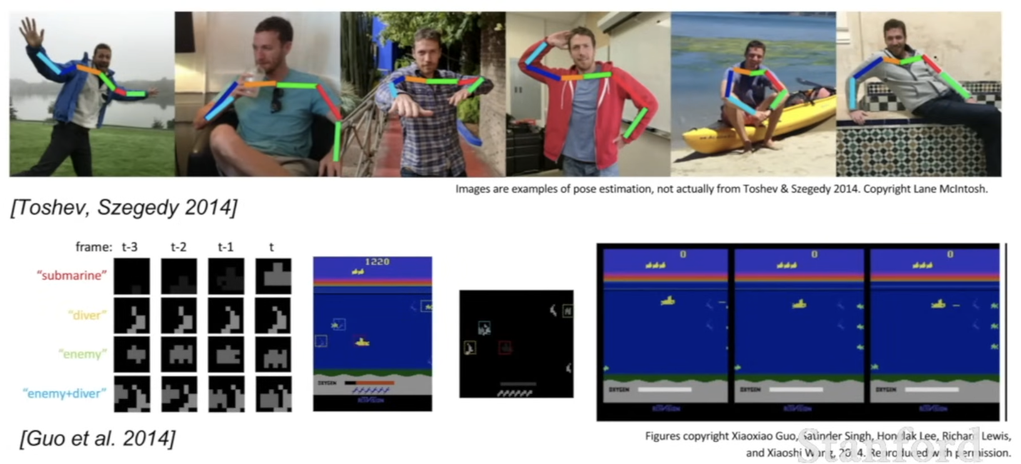
- pose recognition
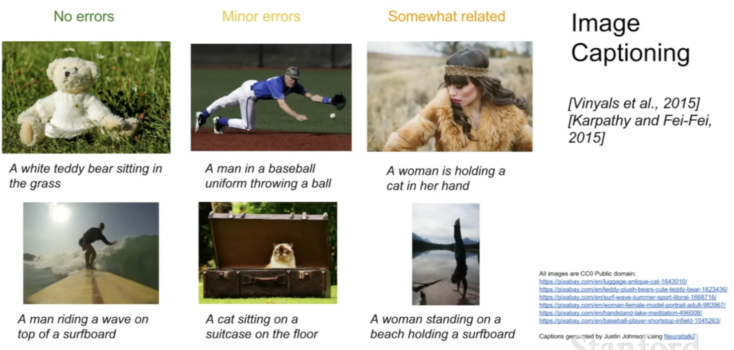
- powered by GPU
Convolutional Neural Networks
Fully Connected Layer
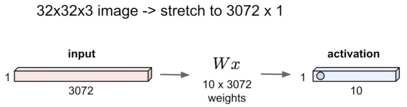
- 3D image of 32x32x3 → stretch all the pixels, get 3072x1 vector
- multiply it by matrix → get activations, the ouput of this layer, in this case take 10 rows and do dot product with 3072 input → 1 number = value of that neuron, we'll get 10 outputs
Convolution layer
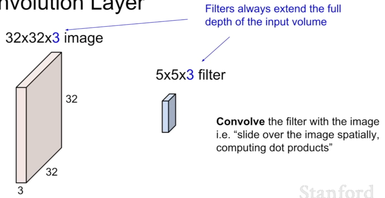
- main difference between fully connected - preserves spatial structure
- instead of stretching this out, keep the structure of this image
- is a small filter, in this case 5x5x3
- filters always extend the full depth of the input volume
- filter = smaller spatial area, but go through the full depth (3)
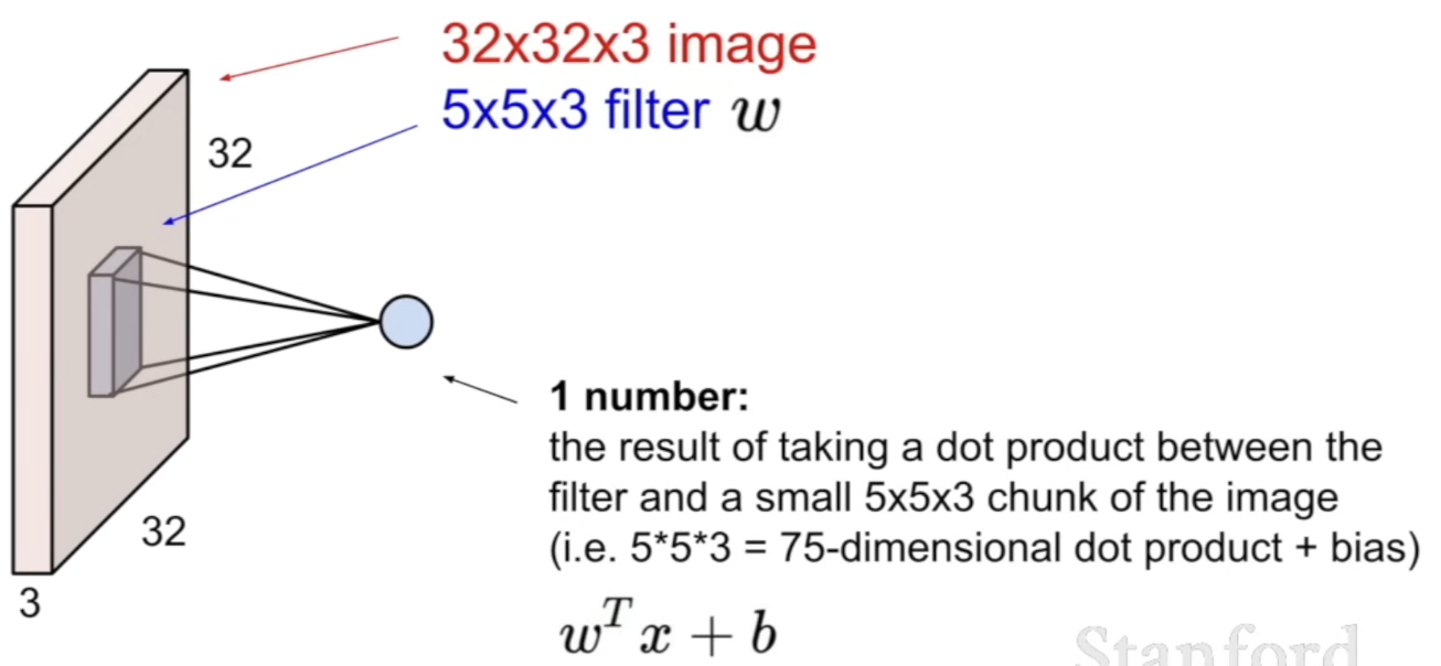
- slide the filter over the image spatially, and do dot products at every space locations
- Why use ?
- just the notation to make the math work out as a dot product
- no intuition here
- take the filters of and stretch it out into a 1D vector, and in order for it to be a dot product, it has to be 1xN vector
- Why use ?
Using one layer
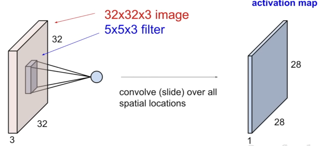
- start at the upper-left corner, center the filter on top of every pixel in this input volume → at every position, do dot product → will produce 1 value in the output activation map
- slide the filter around
- We'll have a choice of how to slide this whether going at every pixel or slide two input values over at a time.. ⇒ you get different sized outputs depending on how you choose to slide
Using multiple layers
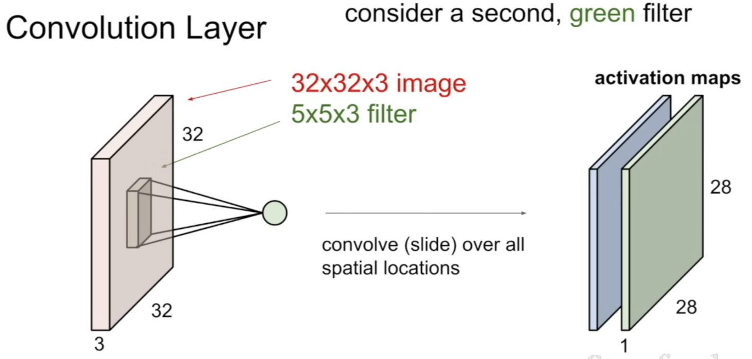
- Now, we want to work with multiple filters
- b/c each filter is looking for a specific type of template or concept in the input volume
- Take the green filter, slide this over the all spatial location, and we get second green activation map of the same size
- We can use as many filters as we want
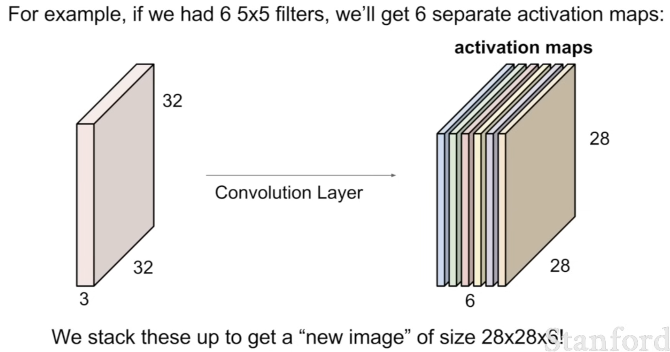
ConvNet
- a sequence of convolutional layers, stacked on top of each other, and intersperse(배치하다) these with activation functions (ex.ReLU activation function)
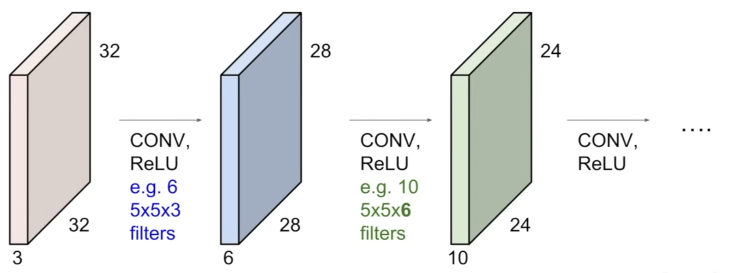
Q: intuition for increasing depth each time?
A: just a design choice, people in practice found out certain types of configurations work better - When using multiple layers stacked in a ConvNet, you end up learning hierarchical filters
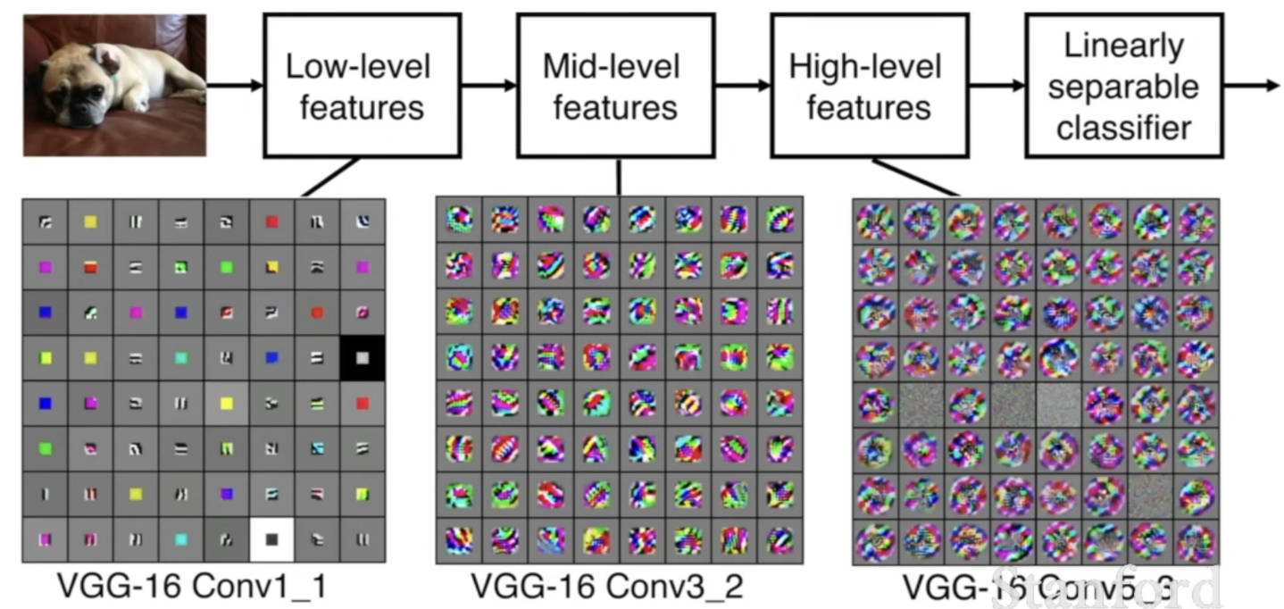
- filters at the earlier layers usually represent low-level features(ex. edges)
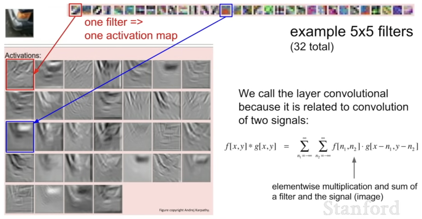
- a row of example 5x5 filters, as we convolve this over an image, each of the activation map is the output of sliding one of these filters
- what these filters are causing are acknowledging where this sort of template is more present in the image
- red box
- template looks like an edge → while sliding over the image, it will have a high value(= more white value) where there are edges in this type of orientation
Q: Why call it convolutional?
A: It's related to the convolution of two signals (convolving with the flipped version of the filter)
- What total convolutional neural networks looks like
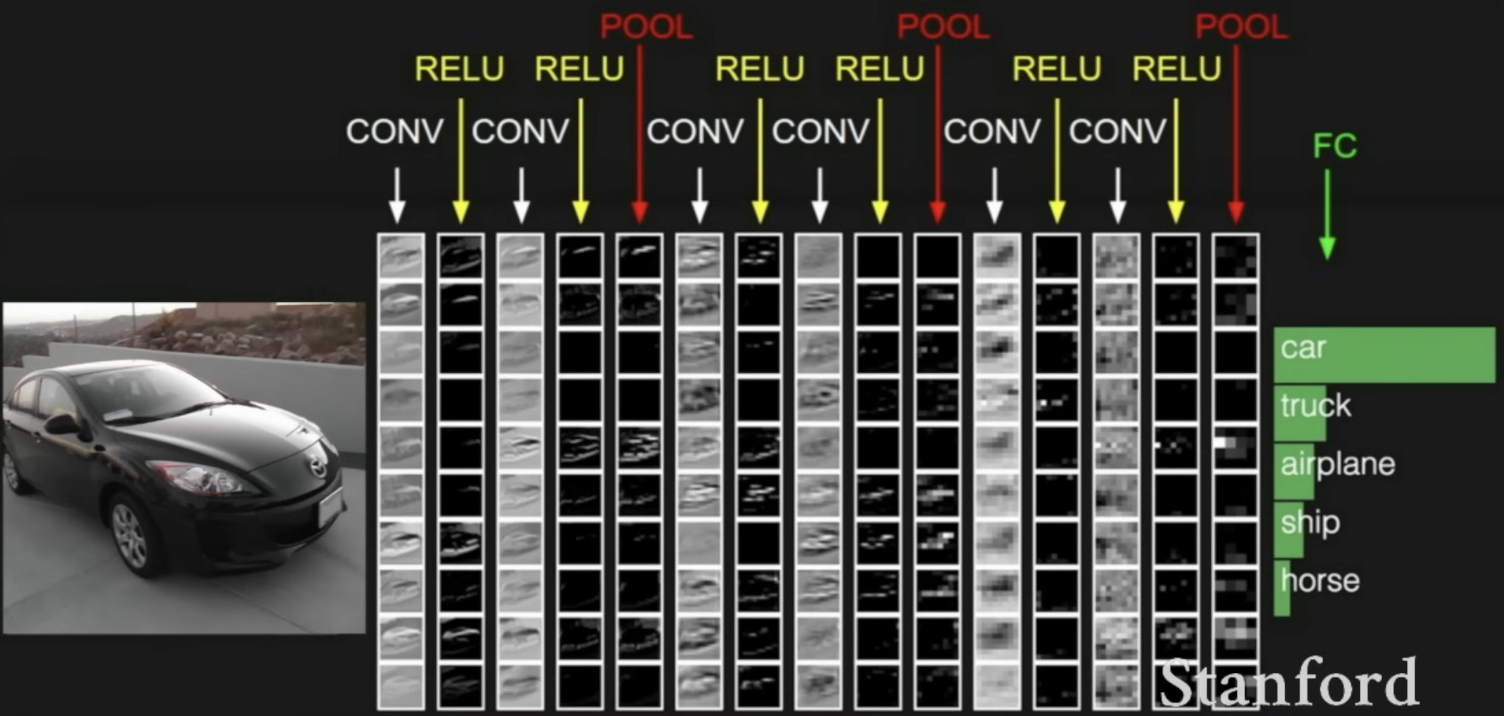
- sequence of layers
- convolutional layer → non-linear layer(ReLU is commonly used) → once in a while, use pooling layer(downsampling the size of the activation map)
Spatial Dimensions
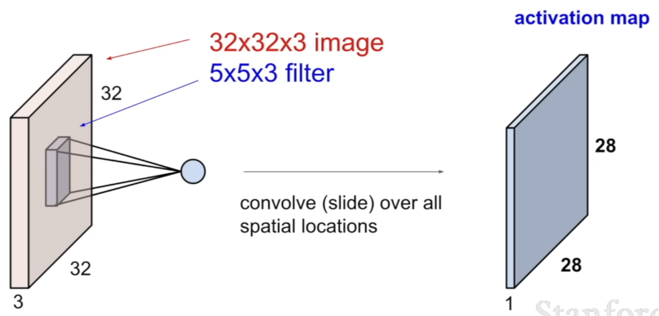
-
how do we end up with 28x28x1 activation map, using 5x5x3 filter?
-
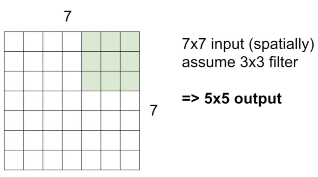
Assume that we have 7x7 input, 3x3 filter
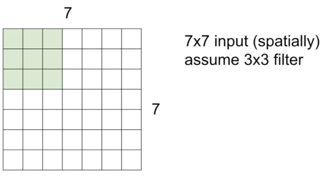
-
put the filter at upper-left corner, and do dot product and get first value → upper left value of the activation map
-
and keep moving
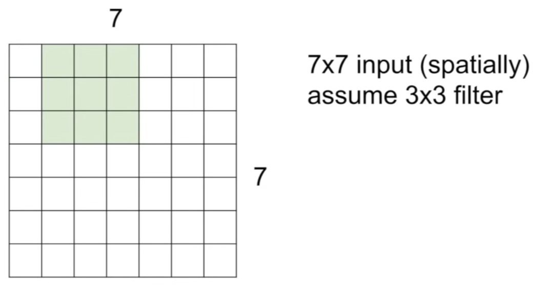
-
We get 5x5 output, b/c what fit was sliding this filter total of 5 spatial locations both horizontally and vertically
Changing Stride and Output size
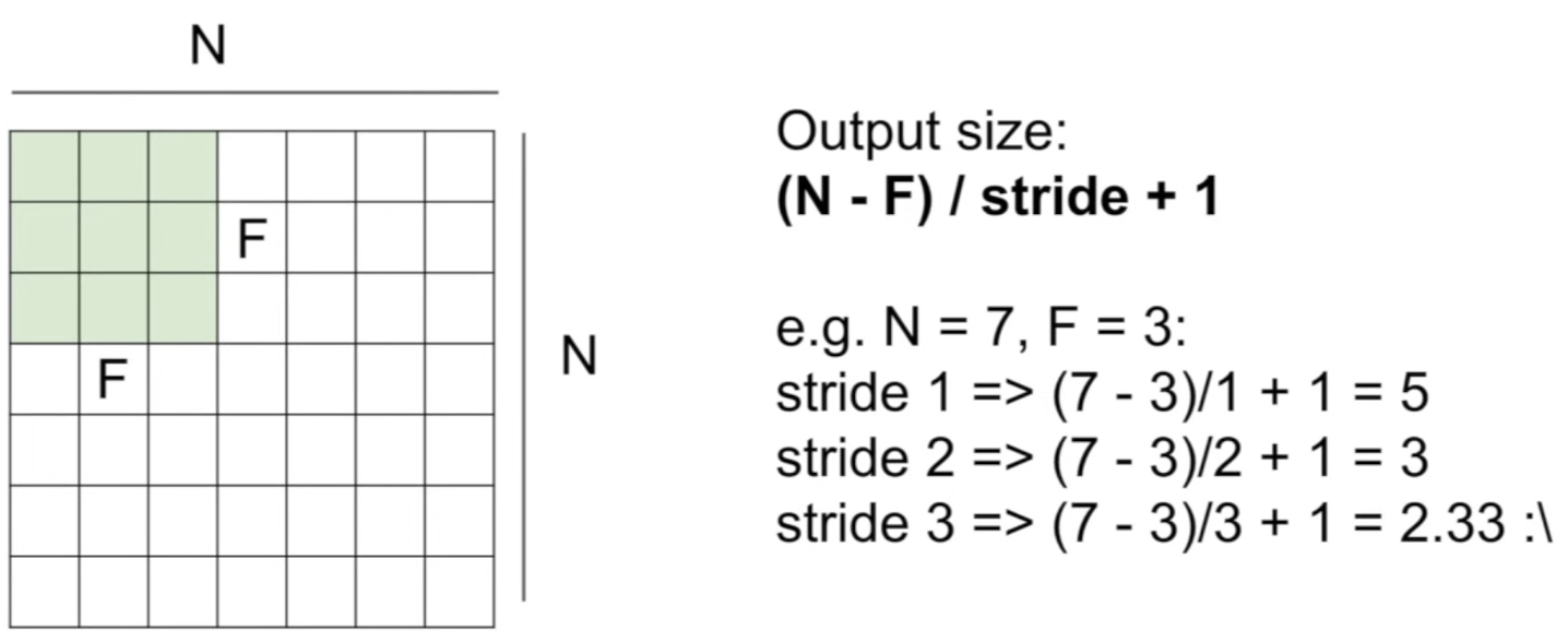
- stride: the interval of sliding the filters
- previously, we used stride of 1
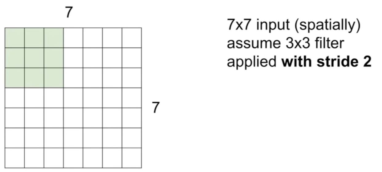
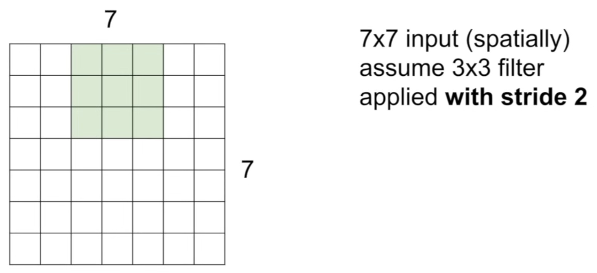
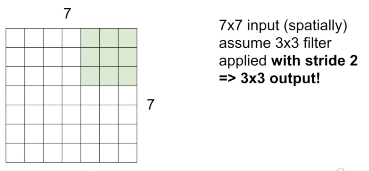
- stride = 2 means skipping 2 pixels over → we have in total 3 of these that can fit, so we get 3x3 output
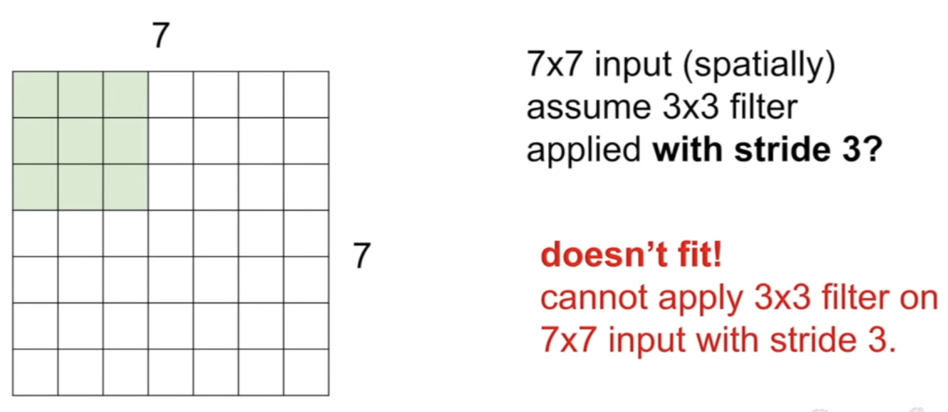
- stride = 3? - doesn't fit, and it will lead to asymmetric outputs
Output size formula
Zero padding the border
- In practice, it's common to zero pad the border
- in order to make the size work out to what we want it to
- to maintain the same input size as we had before (ex. when input is 7x7 and we use 3x3 filter, we get smaller output)
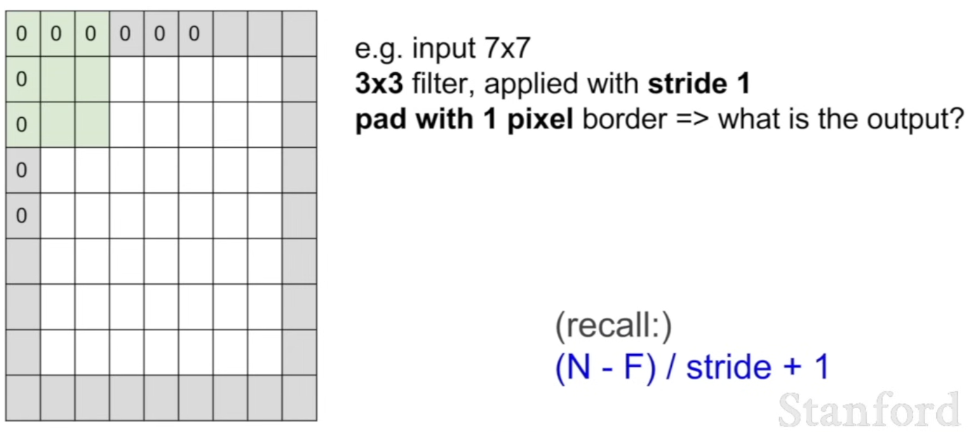
- pad input image with 0s → now able to place a filter centered at the upper right-hand pixel location of the actual input image
- ex) input 7x7, filter 3x3 with stride 1, pad with 1 pixel border → output = 7x7 (b/c now the input is 9x9)
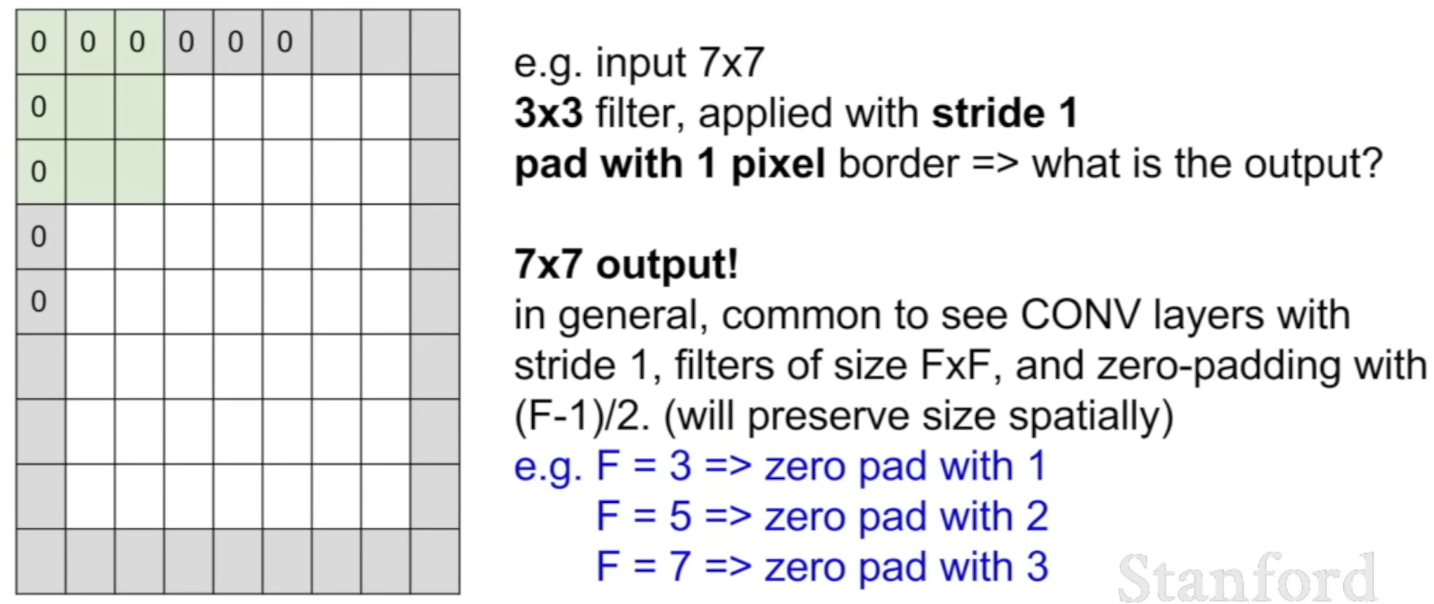
- Why do we use zero pad?
- when we don't, the size of the output shrinks quickly (= not what we want)
- size of the activation map will shrink to somthing very small
- this is bad b/c we're loosing some of the information (end up using much smaller number to represent the original image)
Examples
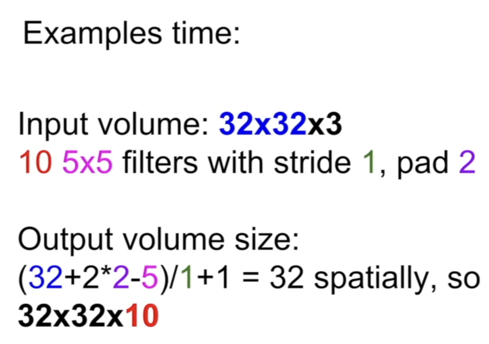
-
Output size?
-
Number of parameters in this layer?
- 760
- each filter has params (+1 = bias term)
- total 10 filters, so
Summary
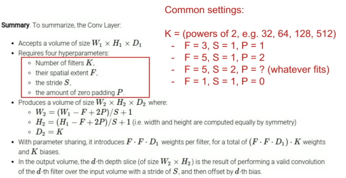
Q: intuition behind choosing the stride?
A: larger stride → end up getting an output of down sampled image (works better sometimes, kind of a pooling in its sense, reducing the size of the activation maps and affects the total number of parameters you get)
- trade-offs between the number of parameters, size of the model, overfitting, etc.
Brain/neuron view of ConV layer
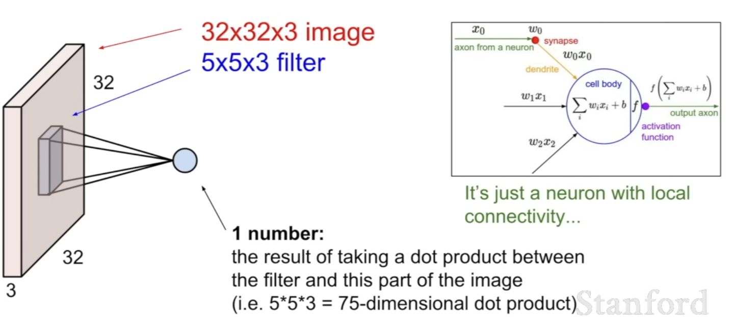
- At every spatial location, we take a dot product between a filter and the specific part of the image, and get 1 number out from here
- Main difference - Neuron now has local connectivity - instead of being connected to the entire input, it only looks at a local region spatially of the image → and get how much this neuron is being triggered at every spatial location of the image
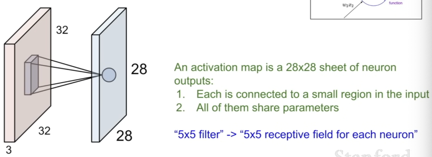
- 5x5 filter = 5x5 receptive field for each neuron
- b/c receptive field = input field that this neuron is receiving
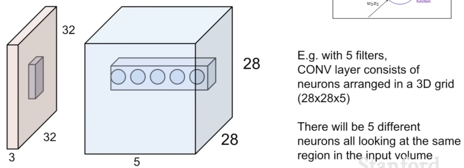
- In one spatial location of the activation volume
- all of these neurons are looking at the same region in the input volume, but looking for different things
- different filters applied to same spatial location in the image
- In Fully Connected Layer,
- each of the neurons in the activation or output was connected to the entire stretched out input
- In Conv layer,
- each neuron is only looking at a local spatial region
Pooling layer
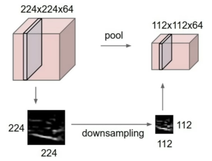
- makes the representations smaller and more manageable
- operates over each activation map independently
- does nothing in the depth, only pooling spatially
- input depth = output depth
Max pooling
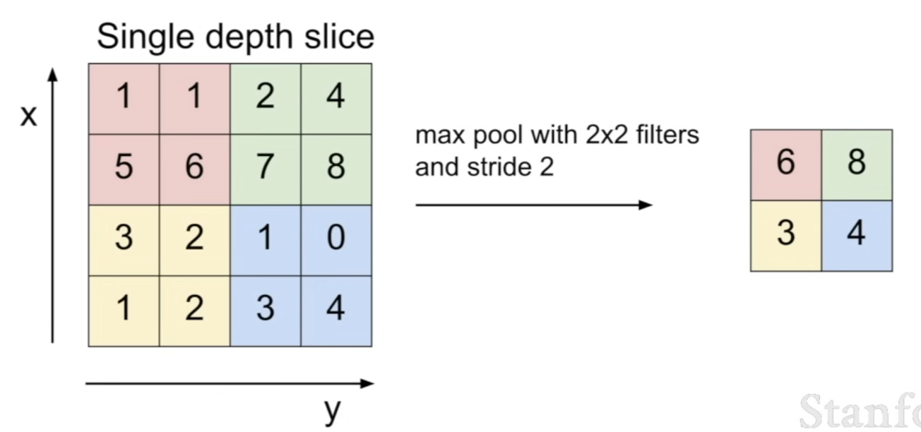
- pooling layer has filter size (= region at which we pool over)
- ex) 2x2 filter and stride 2 → slide it along the input volume, and take the maximum value of the input volume in that region
Q: Is it typical to set up the stride so that there isn't an overlap?
A: Yes, we basically want to downsample, so it makes sense to get a value that represents this one region
Q: Why use max pooling instead of average pooling?
A: Each value in the activation map is how much this filter fired in this location, so think of max pooling saying that giving a signal of how much did this filter fire at any location in this image
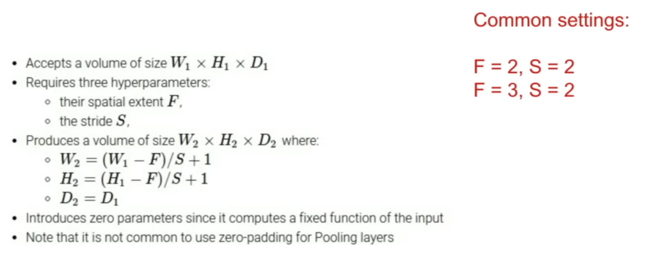
- people don't use zero paddings in pooling layers b/c it's just for downsampling
Fully Connected Layer (FC Layer)
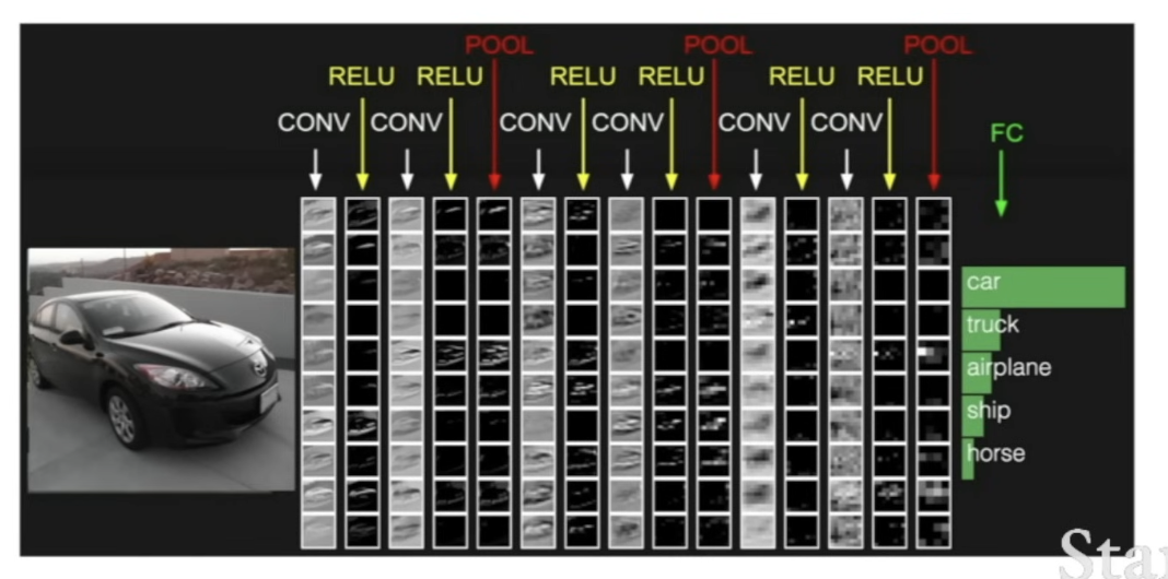
- intersperse these and have a pooling layer every once in a while, and lastly have a fully connected layer
- take the convnet output, stretch these out, and get 1D input and apply this fully connected layer on top
⇒ now have connections to every one of these conv map outputs - We get score ouputs like before
Q: How do we interpret the column, for example at POOL?
A: Each of these columns is the output activation maps / just take the output of the ReLU layer, and downsample it, and take the max value of each location
- looks the same as ReLU output, except it's downsampled and has max value at every spatial location
Q: It looks like small amount of information, how can we classify it from here?
A: each of these values inside one of these pool outputs = accumulation of all the processing you've done throughout this entire network
- as you go thru, it's looking for more complex things (ex. edge → corners)
- by the time you get up to this last pooling layer, each value is representing how much a relatively complex template is firing
Summary
- ConvNets stack CONV, POOL, FC layers
- Trend towards smaller filters and deeper architectures
- Trend towards getting rid of POOL/FC layers (just CONV)
- Typical architectures look like
- [(CONV-RELU)*N-POOL?]*M-(FC-RELU)*K, SOFTMAX
where N is usually up to ~5, M is large, 0<=K<=2 - but recent advances such as ResNet/GoogLeNet challenge this paradigm
- [(CONV-RELU)*N-POOL?]*M-(FC-RELU)*K, SOFTMAX
