🔎 Stanford CS231n 강의를 듣고 기록용도로 정리하는 게시글입니다.

Activation Functions

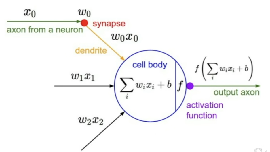
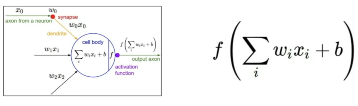
• At any particular layer, data comes in, multiply by weight, pass this through an activation function or nonlinearity

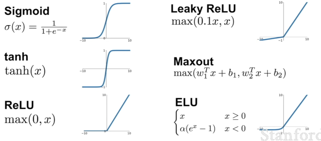
Sigmoid Function

• $\sigma(x) = \displaystyle\frac{1}{1+e^{-x}}$
• Squahses numbers to range [0,1]
• Historically popular since they have a nice interpretation as a saturating "firing rate" of a neuron

Problems

1. Saturated neurons 'kill' the gradients
   

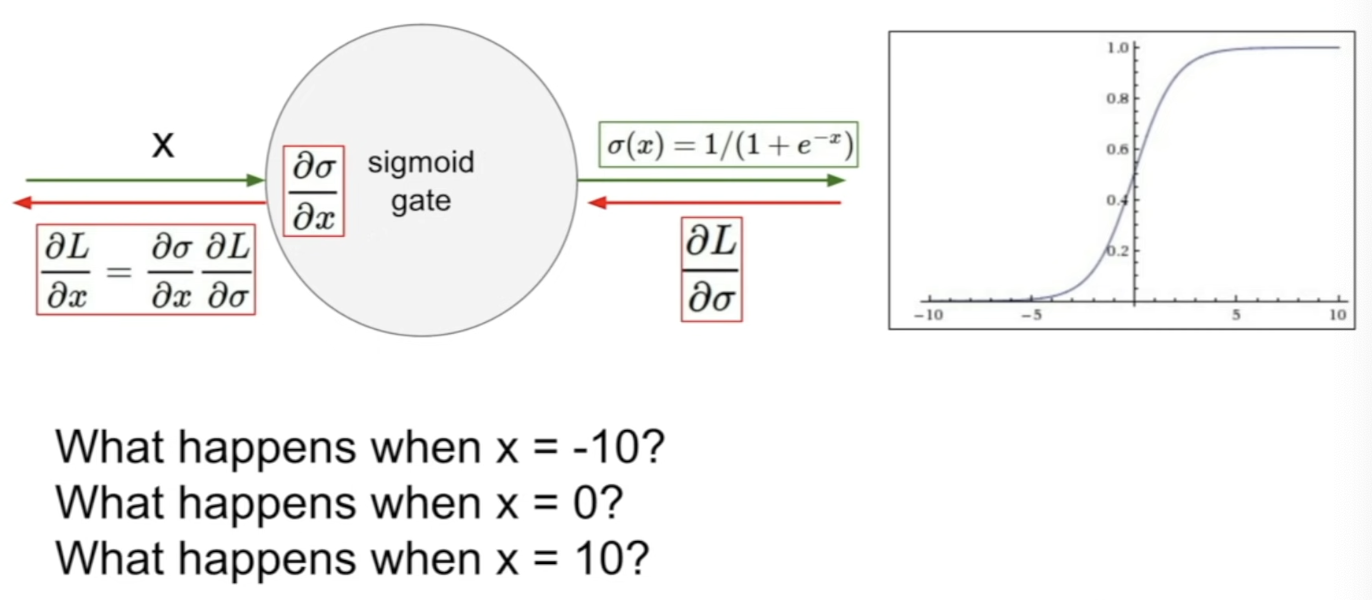
   • when coming back, upstream gradient(= $\displaystyle\frac{dL}{d\sigma}$), multiply it by local sigmoid function(= $\displaystyle\frac{d\sigma}{dx}$), pass back the output
   • What happens when x = -10?
     • gradient = 0
     • b/c in the negative region of sigmoid, it's essentially flat, so the gradient = 0
     • as a result we'll get a very small gradient that's flowing backwards
     • after the chain rule, this kills the gradient flow, and we'll have 0 gradient passed down to downstream nodes
   • What happens when x = 0?
     • we'll get a reasonable gradient
   • What happens when x = 10?
     • gradient = 0 (x의 절댓값이 커지면 함수의 기울기가 결국 0이 되기 때문에 $d\sigma$값이 0에 가까워지기 때문)
     • regions where sigmoid function is flat
     • will kill the gradient flow and won't get a gradient flow coming back

2. Sigmoid outputs are not zero-centered

   • Consider what happens when the input to a neuron (x) is always positive
     
   • What can we say about the gradients on $W$? (in this case, say all the xs are positive)
     
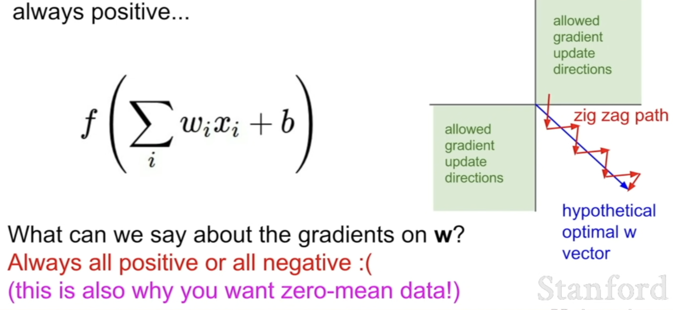
   • Always all positive or all negative
     • upstream gradient = $\frac{dL}{dF}$ → this will be either positive or negative
     • local gradient = $\frac{dF}{dW} = x$ → if $x$ is always positive, then the gradients on $W = \text{upstream gradient} \times \text{local gradient}$ = sign of the upstream gradient coming down
     • this means that all the gradients on $W$, since they're always either positive or negative, they're always going to move in the same direction = when doing an update, you'll either increase all of the values of $W$ by a positive amount or decrease them all
     • problem - gives very inefficient gradient update
   • ex) $W$ is 2D (2 axes), say that we can only have all positive or all negative updates
     • if blue vector is the hypothetical optimal $W$ vector, we can't just take a gradient update in this direction
     • b/c this is not in one of those 2 allowed directions
     • so, we'll have to take a sequence of gradient updates (ex. red arrow directions)
   • This is why we want the input $X$ to be zero meaned, so that we actually have positive and negative values and not get in the problem of gradient updates being moved in same direction

3. exp() is a bit compute expensive

   • just a minor point to observe (b/c convolutional layers and dot products are a lot more expensive)

tanh(x) function

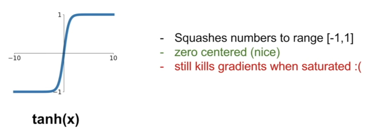
• still have regimes where the gradient is essentially flat → kills the gradient flow
• bit better than sigmoid, but still has problems

ReLU function

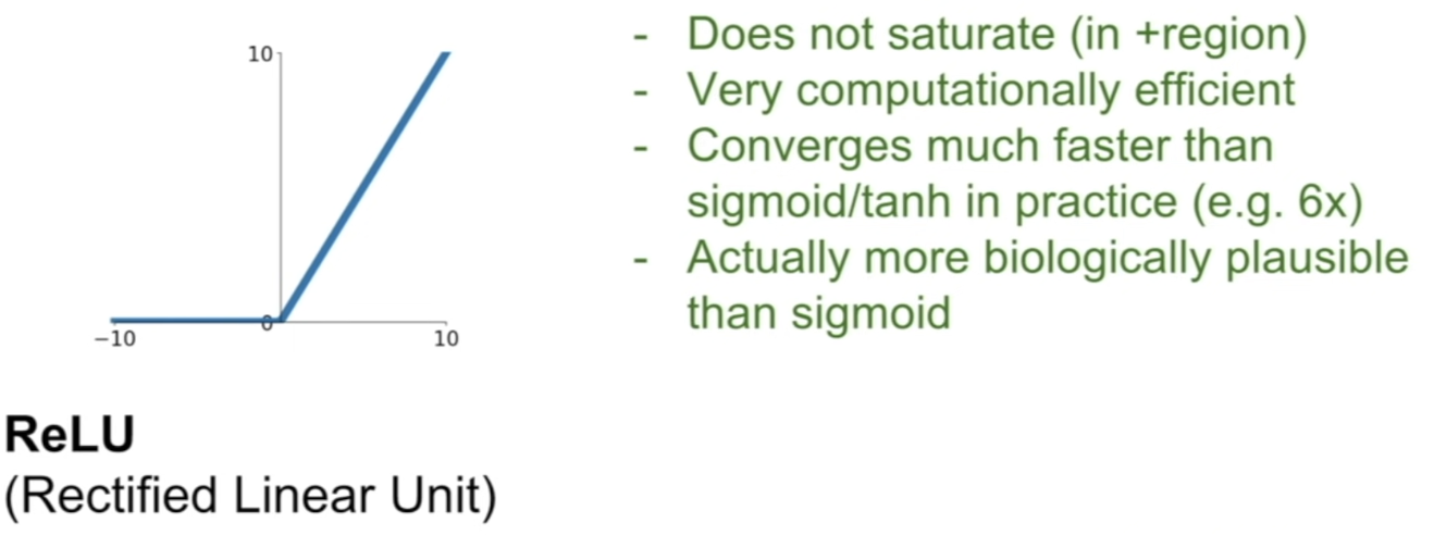
• $f(x) = max(0,x)$ (Rectified Linear Unit)
• if input is negative, put it to 0, if it's positive, just pass it through
• BUT
  • not zero-centered output
  • an annoyance
    • in the positive half of the inputs, no saturation
    • in the negative half of the inputs, it's not the case

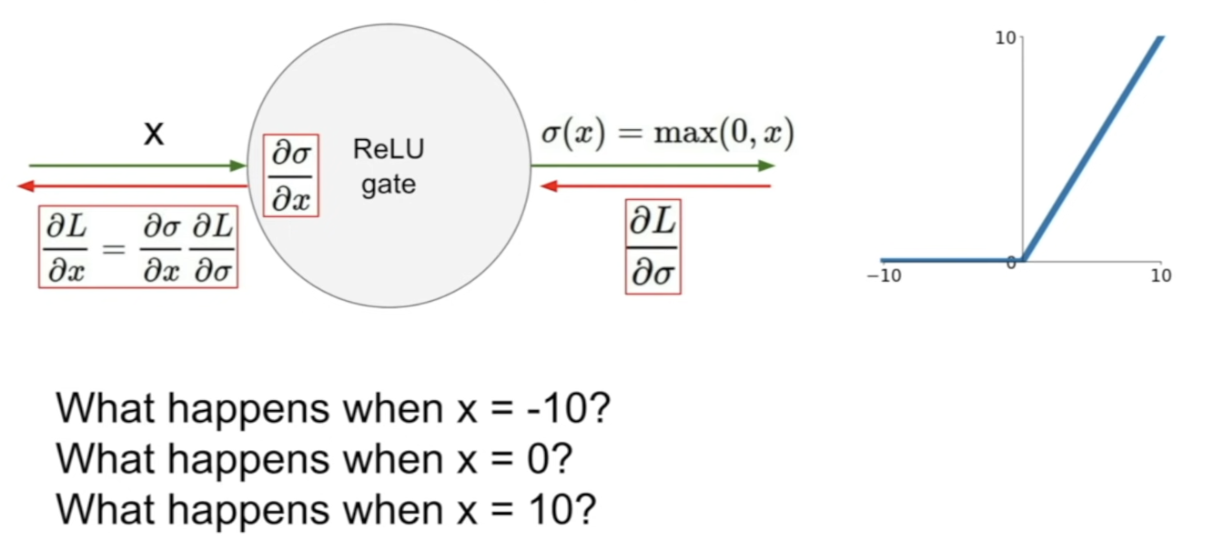
• x = -10?
  • gradient = 0
• x = 10?
  • linear regime
• x = 0?
  • undefined, but in practice we'll say it's 0
• it's killing the gradient in the half of the regime

Dead ReLUs

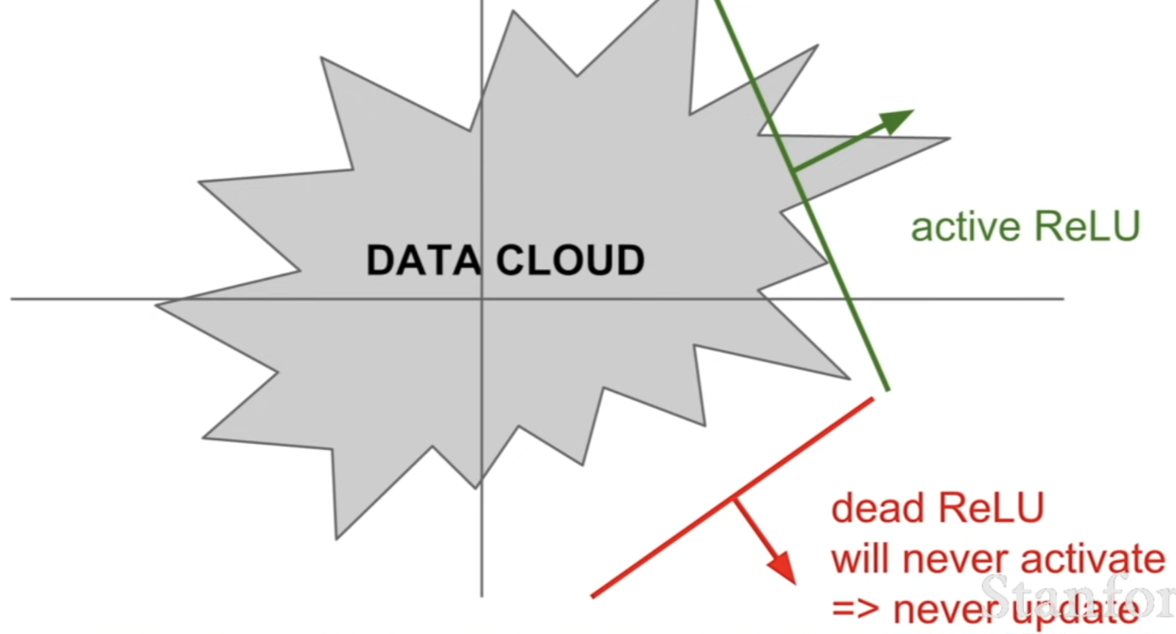
(data cloud = training data)

• dead ReLUs are off of the data cloud, in this case it will never update

• compared to active ReLU, some of the data will be positive and passed through, and some won't be

• Reasons
  1. Bad Initialization

  • weights that happen to be unlucky, be off the data cloud → so they happen to specify the bad ReLU
  • they're never going to get a data input that causes it to activate, so they will never get good gradient flow coming back, so it'll never activate and update
  2. Too High Learning Rate
  • start off with okay ReLU, but b/c you're making huge updates → weights jump around → ReLU unit gets knocked off of the data manifold
  • happens through training

Q: How do you tell when the ReLU is going to be dead or not, with respect to the data cloud?
A: We'll get input to the ReLU, which is going to be $W_1 \times x_1 + W_2 \times x_2$ → apply this → that defines this separating hyperplane → take the half which will be positive, and half of it will be killed off

Q: In sigmoid, one of the drawbacks was that the neurons can get saturated
A: In sigmoid, when all of the inputs are positive, they're all going to be coming in the 0+ region, so you still get a saturating neuron b/c up in the positive region, it plateaus at 1. So, when you have large positive values as input, you'll get the 0 gradient b/c you have a flat slope here.

• some people like to initialize ReLU neurons with slightly positive biases (ex. 0.01)
  - in order to increase the likelihood of it being active at initialization and to get some updates
  - this biases toward more ReLUs firing at the beginning
  

Modified ReLUs

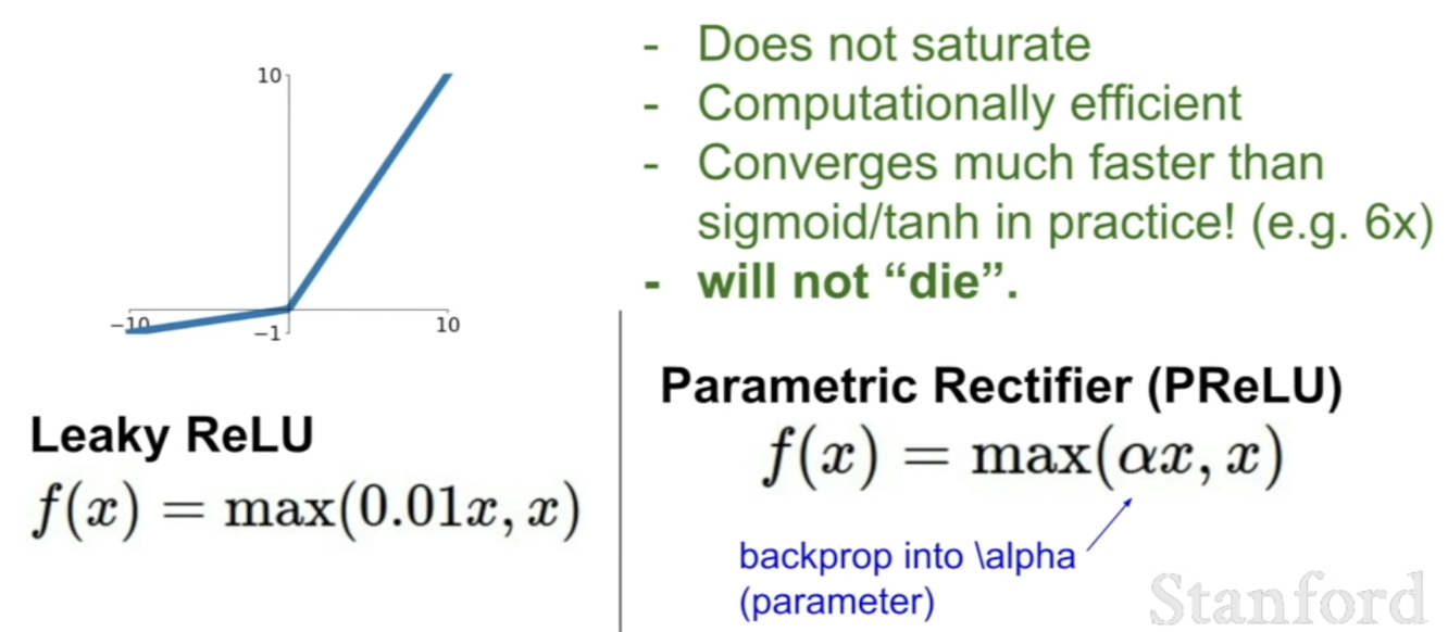
Leaky ReLU

• instead of being flat in the negative regime, it gives a slight negative slope here
• no saturation even in the negative regime

PReLU (parametric rectifier)

• just like leaky, has a sloped region in the negative space
• slope in the negative regime is determined through $\alpha$ parameter
  • treat it as a parameter that we can backprop and learn
• more flexibility

ELU (Exponential Linear Units)

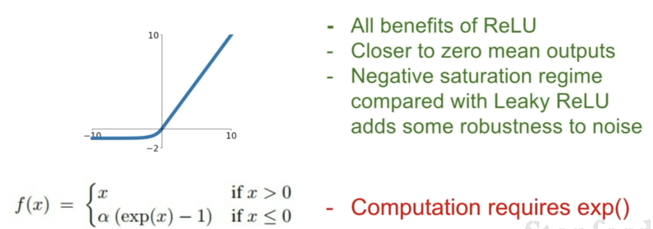
• something in between the ReLU and the leaky ReLU

Maxout "Neuron"

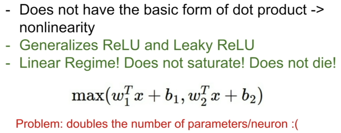
• take the max of these 2 functions
• kind of generalizing the ReLU and the leaky ReLU b/c it's taking the max over these 2 linear functions
• BUT each neuron has $W1$ and $W2$ → twice of the original Weight

TLDR: In practice:

• Use ReLU. Be careful with learning rates
• Try out Leaky ReLU / Maxout / ELU
• Try out tanh but don't expect much
• Don't use sigmoid

Data Preprocessing

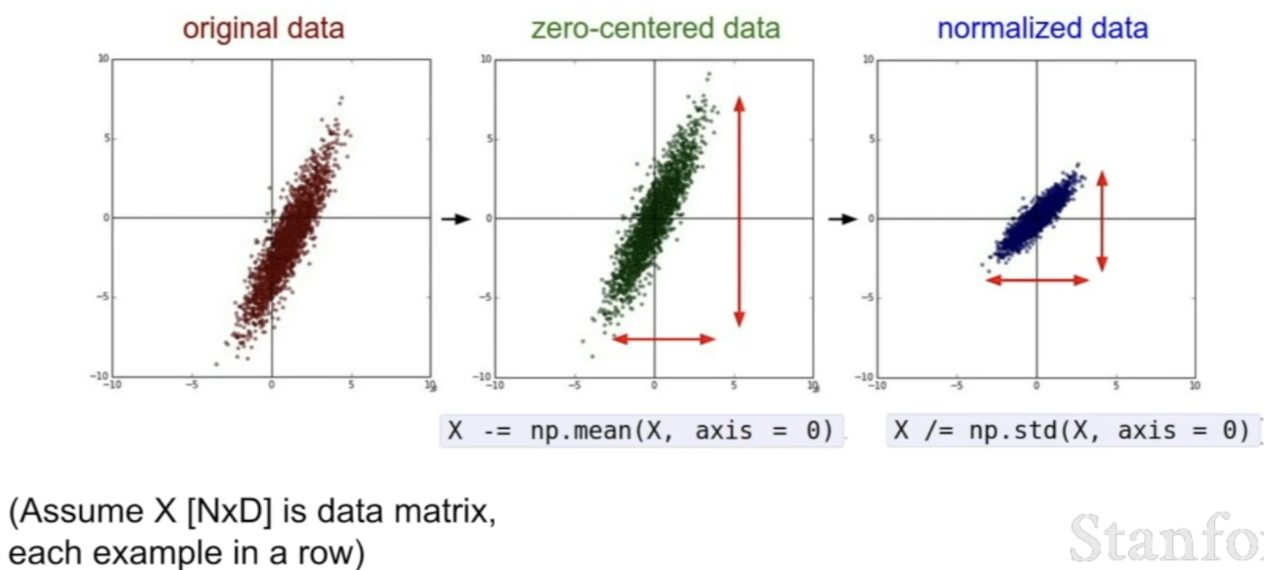
• some standard types of preprocessing: take data, zero mean them, normalize them (by standrad deviation)

Zero meaning the data

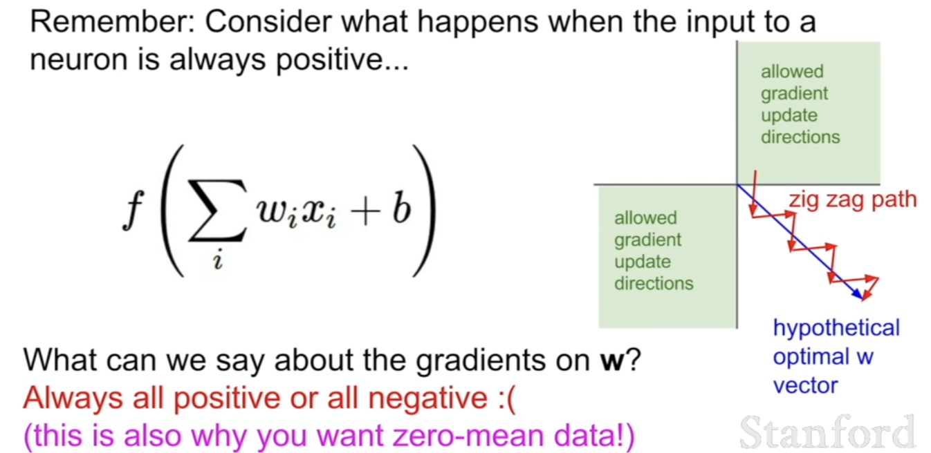
• Why do this?
  • remember that when all the inputs are positive, we get all the gradients on weights to be positive, and we get the suboptimal optimization
  • in general, even if it's not all 0 or all negative, any sort of bias will still cause this problem

Normalizing the data

• ensure that all feature are in the same range, so that they contribute equally
• if data = image
  • in practice, we do do the zero centering but not normalization (pixel values)
  • b/c for images, at each location, you already have relatively comparable scale and distribution

PCA, Whitening

• with images, typically just stick with the 0 mean, don't do complicated preprocessing
  • b/c we don't want to take all the input(pixel values), and project this onto a lower dimensional space of new kinds of features
  • just want to apply convnets spatially and have spatial structure over the image

Q: Do we preprocess data in the test phase?
A: Yes.

TLDR: In practice for images

• CENTER ONLY
• e.g. consider CIFAR-10 example with [32, 32, 3] images
  • Subtract the mean image (e.g. AlexNet)
    (mean image = [32, 32, 3] array)
  • Subtract per-channel mean (e.g. VGGNet)
    (mean along each channel = 3 numbers)
    • just taking the mean by channel
    • b/c it turns out that it was similar enough across the whole image, it didn't make such a difference to subtract the mean image vs. just a per-channel value
    • easier to pass around and deal with
  • do the same thing at test time for this array you deteremined at training time
• NOT common to normalize variance, to do PCA or whitening

Q: What is a channel?
A: channel = RGB. here, the depth, we have 3 channels = RGB → 1 mean for the red channel, 1 mean for the green, blue

Q: when we are subtracting the mean image, what is the mean taking over
A: mean is taking over all of the training images. Take all of the training images and compute the mean of all of those.

Q: Does the data preprocessing solve the sigmoid problem?
A: It does solve this for the 1st layer so the inputs for the first layer will be 0 mean. But this problem will come up in much worse and greater form as we have deep networks. Not sufficient.

Weight Initialization

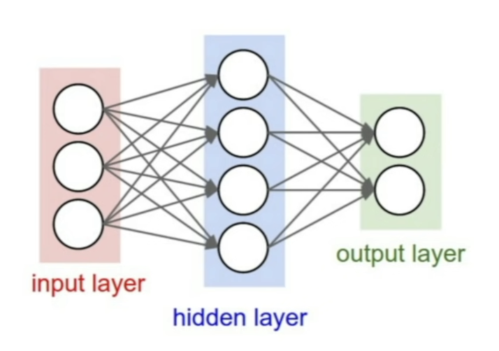
• Say that we have a standard 2 layer neural network and we have weights that we want to learn.

  • But we have to start them with some value (will update them using the gradient updates from there)

• What happens when $W=0$ init is used?

  • neurons will all do the same thing.
  • every neuron is going to have the same operation on top of the inputs
  • they'll all output the same thing, so they'll all get the same gradient
  • so, they'll update in the same way, and all the neurons will be exactly the same != not what we want(we want the neurons to learn different things)

Q: Because the gradient depends on the loss, won't one backprop differently compared to the other?
A: In the last layer, yes. But generally throughout the network, all the neurons are connected in exactly the same way, same update → going to be a problem

First idea; Small random numbers

• gaussian with zero mean and 1e-2(=0.01) standard deviation
  • gives us many small ramdom weights

W = 0.01* np.random.randn(D,H)

• does work okay for small networks
• but problems with deeper networks
  
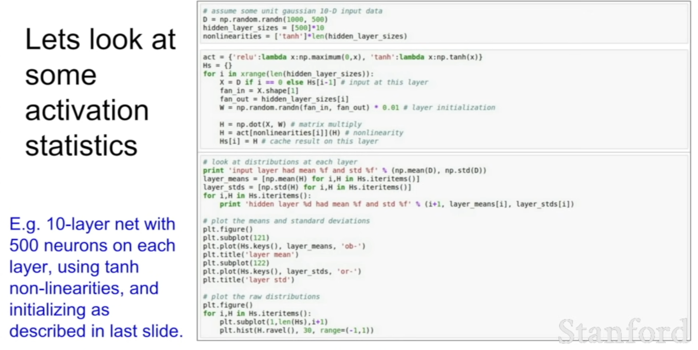
• initialize it with small random numbers

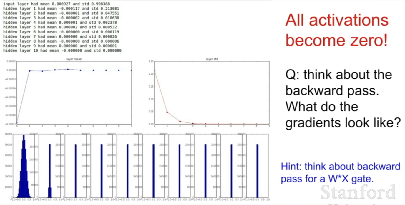
• if we compute the mean and the standard deviations at each layer,

  • 1st layer outputs: means are always around 0 (makes sense)
    • b/c tanh is centered around 0
    • but standard deviation shrinks, quickly collapses to 0
  • Bottom graph is the distribution of the activations we have
    • as we multiply by this $W$ (small numbers), this quikcly shrinks and collapses all of these values as we multiply this over and over again
    • by the end, we get all 0 → not what we want

• Consider backwards pass

  • input values are very small at each layer (b/c they all collapsed at this near 0)
  • now each layer has upstream gradient flowing down, in order to get the gradient on weights = upstream gradient x local gradient ⇒ going to be $X$ (=inputs)
    • b/c $x$ is small, weights are getting a very small gradient, so they're basically not updating
  • basically, when doing backward pass, we're multiplying by $W$ over and over again, we're getting the same phenomenon as we had in the forward pass (everything is getting small and smaller, and the upstream gradients are collapsing to 0 as well)

Second idea; Making weights big

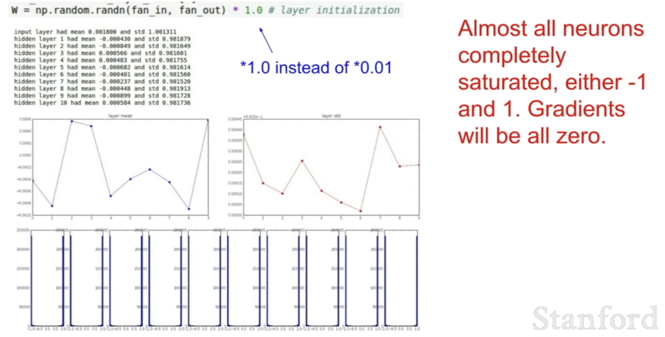
• sample from standard gaussian, standard deviation of 1
• taking the $W \times x$ outputs and passing them through $\tanh$ nonlinearities
  • problem - it's going to saturated
  • now, because our weights are big → we're always going to be at saturated regimes of either very negative or very positive of $\tanh$
• look at the distribution of the activations of each layers
  • will all be -1 or +1
  • so, this will have the $\tanh$ problem; when saturated, all the gradients will be 0, gradients not updating

Xavier initialization

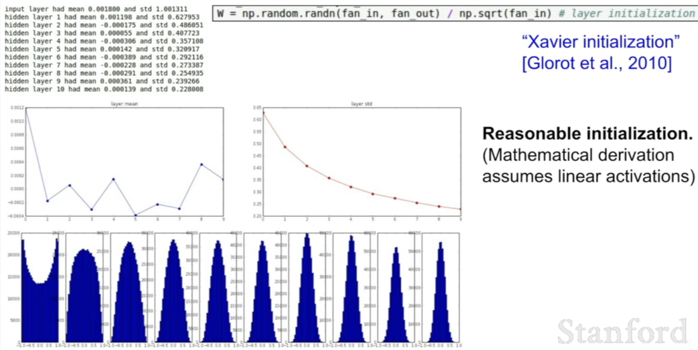
• initialize $W$ = sample from standard gaussian, scale by the number of inputs

• specify that we want the variance of the input to be the same as a variance of the output

• this intuitively means that if you have a small number of inputs, we'll divide by the smaller number and get larger weights

  • we need larger weights b/c we'll multiply those small inputs by weight, and you need larger weights to get the same larger variance at output
  • if we have many inputs, we want smaller weights
    • in order to get the same spread at the output

• this assumes that there's linear activation (= active region of the activation)

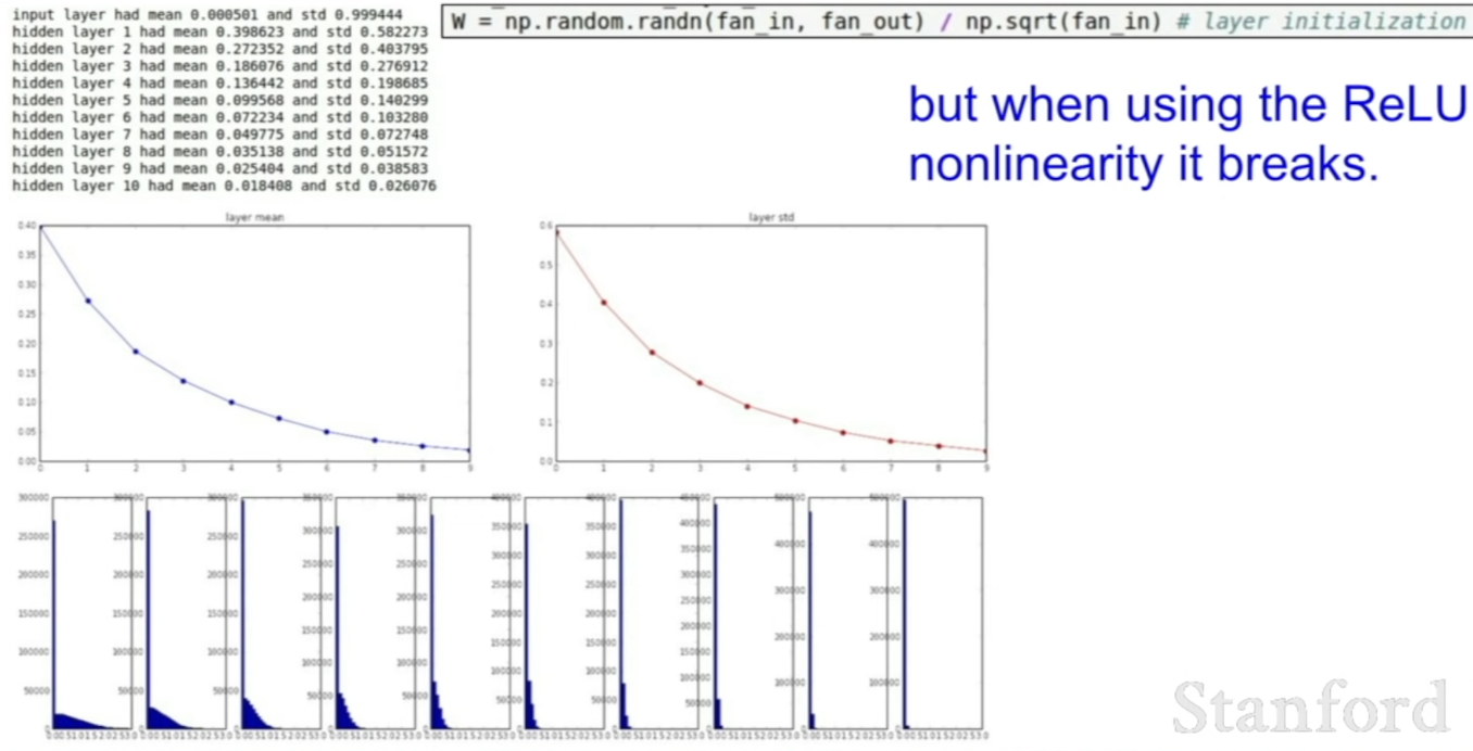
• Problem: breaks when using ReLU
  • b/c it's killing half of your units, it's setting approximately half of them to 0 at each time
  • it's halving the variance that you get out of this
  • distribution starts collapsing

Extra 'divided by 2'

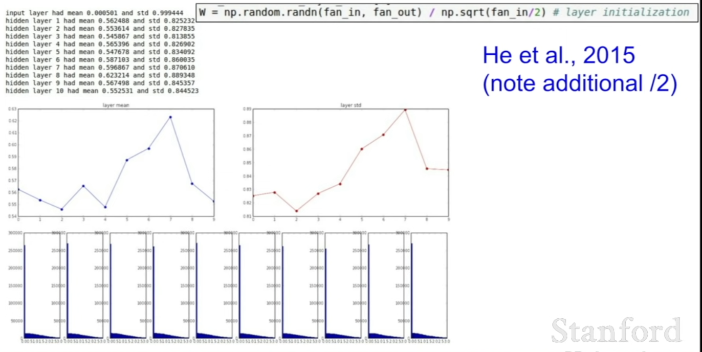
• adjusting the fact that half the neurons get killed
• works much better
• distributions are pretty good throughout all layers of network

Batch Normalization

• if we want unit gaussian activation, let's force them to be that way
• consider a batch of activations at some layer
  
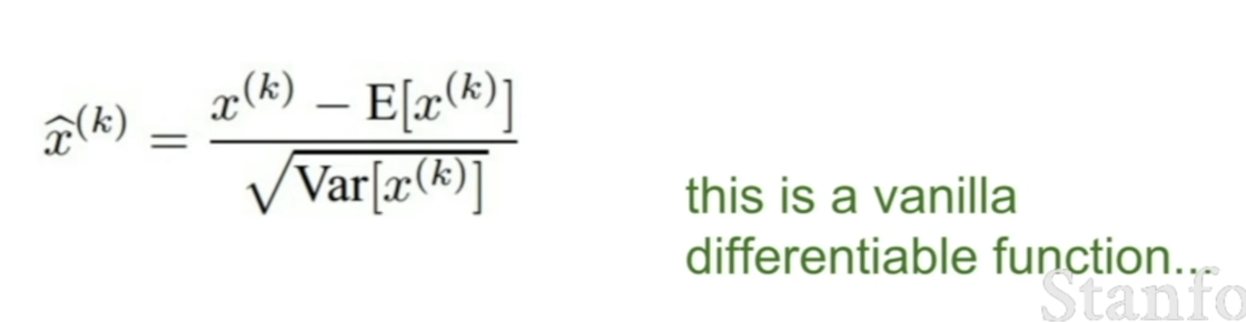
  • explicitly make every layer have unit gaussians without weight initialization happening on every forward pass through the network
  • by normalizing by the mean and the variance of each neuron, look at all of the inputs coming in, and calculate the mean and variance for that batch, and normalize by it
    • this is just a differentiable(미분 가능) function
  • if we have the mean and variance as constants

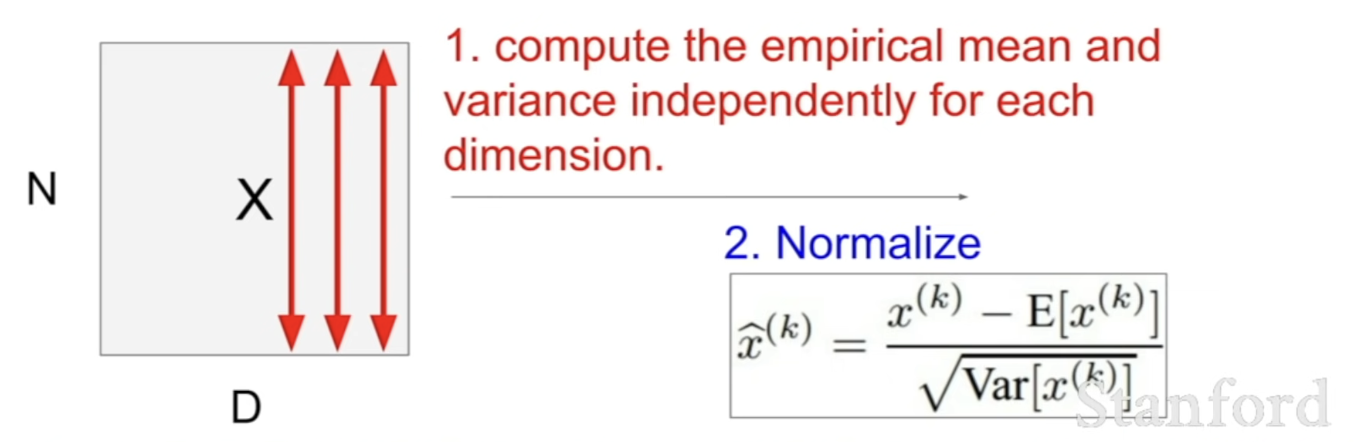
• N training examples in current batch, each batch has dimension D

1. compute the empirical mean and variance independently for each dimension
   • compute this across our batch
2. normalize by the current mini-batch

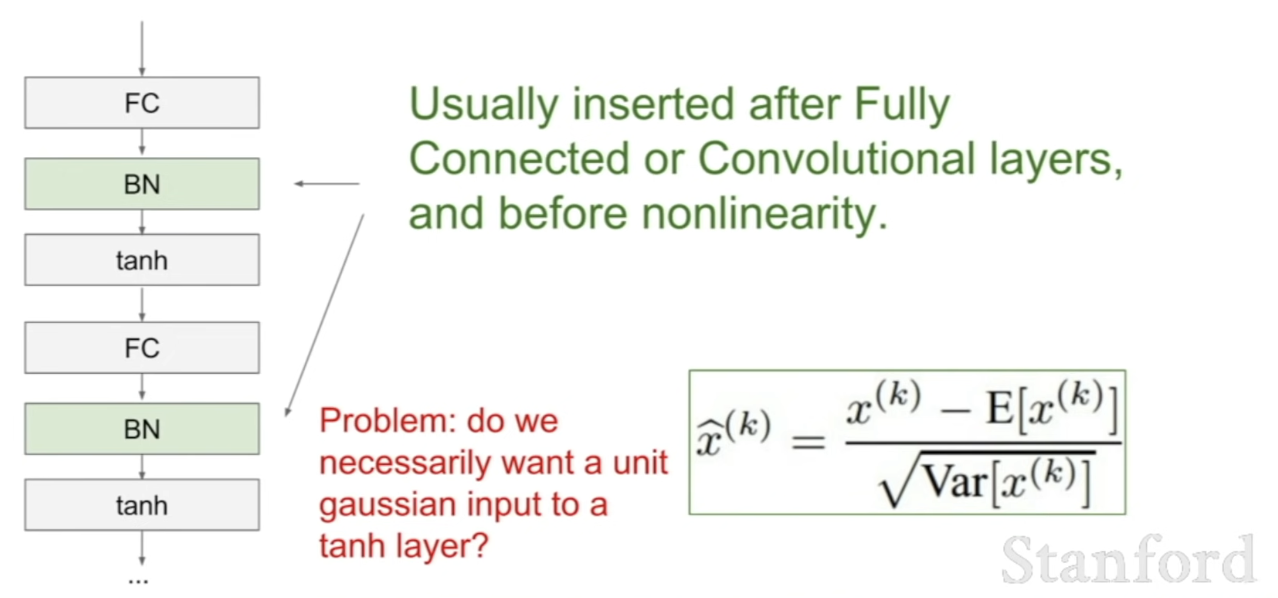
• able to undo the bad scaling effect that happens when we're multiplying $W$ over and over again

• basically scaling by the inputs connected to each neuron, each activation → apply this the same way to FC and Conv layers

  • only diff: with conv, we want to normalize not just across all the training example, and independently for each feature dimension, but want to normalize jointly across both of all the feature dimensions, all the spatial locations we have in our activation map as well as all of the training example
  • in conv layer, have 1 mean and 1 standard deviation per activation map, and normalize by this across all of the examples in the batch

• Problem: it's not clear that we necessarily want a unit gaussian input to these tanh nonlinearities

  • b/c this is constraining you to the linear regime of this nonlinearity
  • BUT you want to control how much saturation you want to have

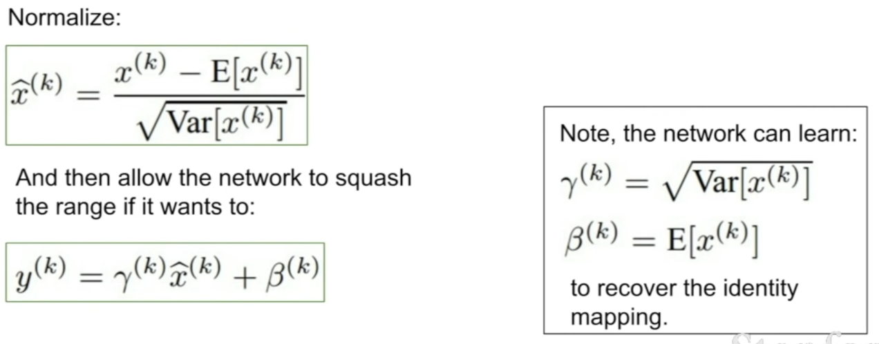
• after normalization, we have an additional squashing and scaling operation (scale by some constant $\gamma$, and shift by another factor of $\beta$)
  • it allows you to be able to recover the identity function if you want to
  • if the network wants, it could learn the scaling factor $\gamma$ to be your variance, $\beta$ to be your mean, in this case you can recover the identity mapping as if you didn't have batch normalization
  • now you have the flexibility of doing everything in between, and make the network to learn how to make the tanh more or less saturated, and how much to do so in order to have good training

Summary

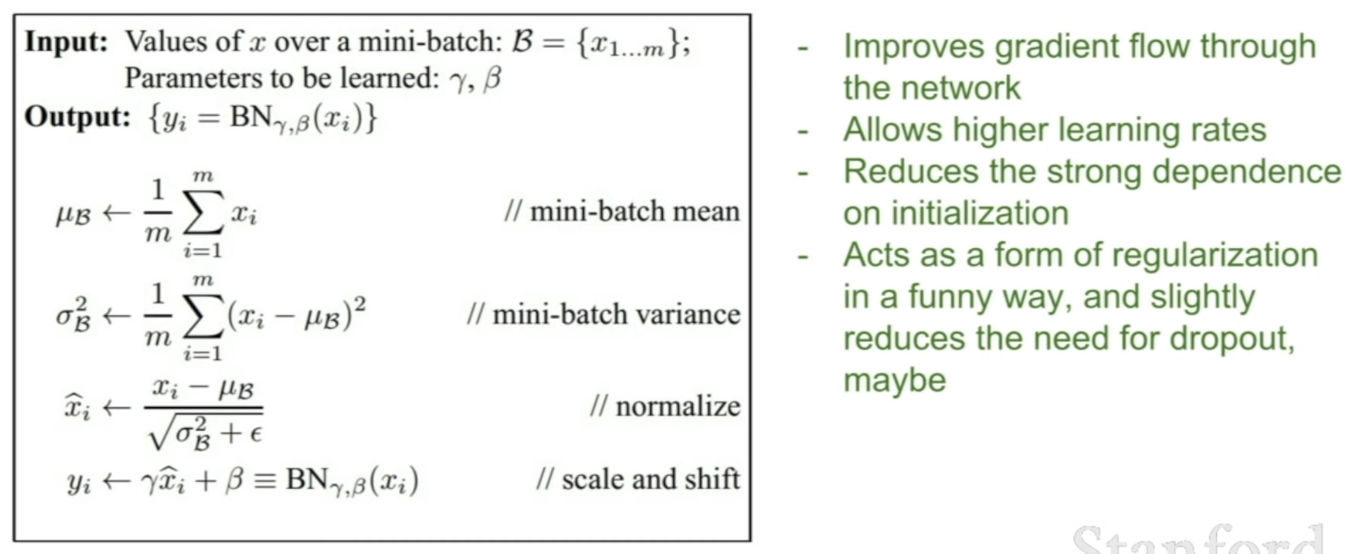
• compute our mini-batch mean, for every mini-batch
• compute variance
• normalize by this mean and variance
• additional scaling and shifting factor
• improves gradient flow through the network, and more robust
  • works for more range of learning rates, and different kinds of initialization
• can think of this in a way of doing regularization
  • b/c now at the output of each layer, each of these outputs is an output of both input X as well as the other examples in the batch
    • b/c normalize each input data by the empirical mean over that batch
  • no longer produces deterministic values for a given training examples, and it's trying all of these inputs in a batch together
  • jitters the representations of X a little bit= give some regularization effect

Q: Why do we want to learn the gamma and beta to be able to learn the identity function back?
A: for flexibility. what batch normalization is doing is forcing our data to become unit gaussian. even though in general this is a good idea, it's not always the best thing to do

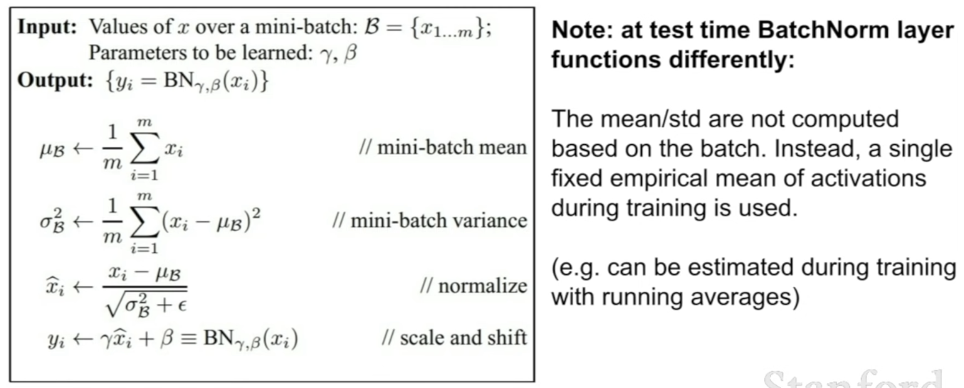
• at test time, the batch normalization layer, take the empirical mean and ㅍㅁvariance from the training data
  • we don't re-compute this at test time, just estimate this at training time (ex. using running averages)
  • use this at test time

Babysitting the Learning Process

• how do we monitor training, adjust hyperparameters as we go to get good learning results?

Step 1; Preprocess the data

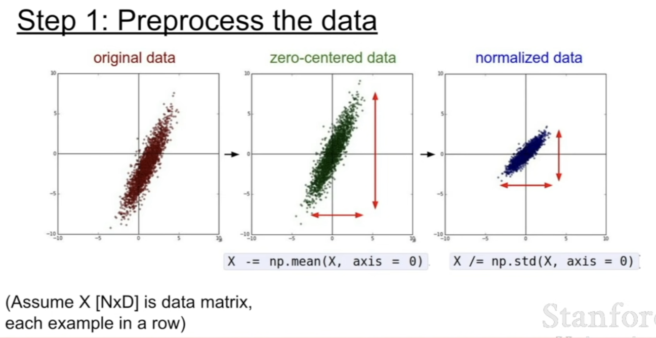
• zero-mean the data

Step 2; Choose the architecture

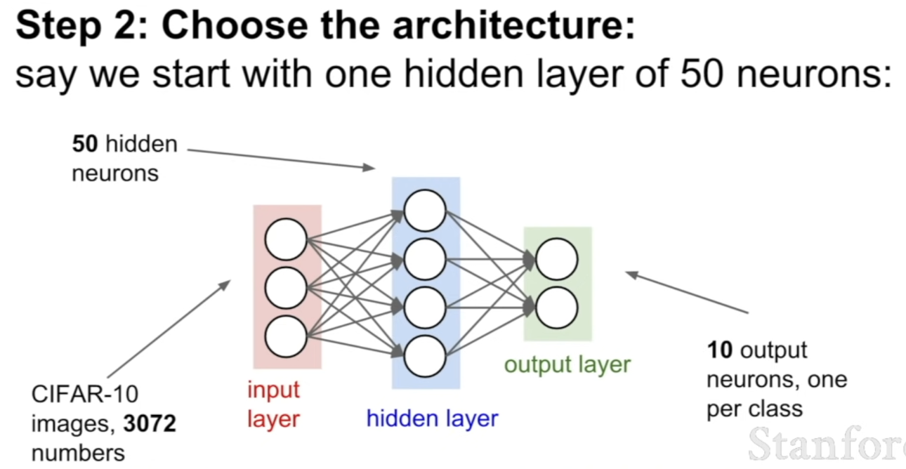
• here, we're starting with 1 hidden layer with 50 neurons
• but we can pick any structure

Step 3; Double check the loss

• initialize the network, do a forward pass through it, and make sure that the loss is reasonable

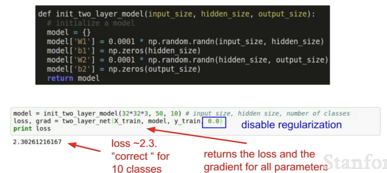
• say that we have a softmax classifier
  • we know what our loss should be when our weights are small and we have generally a diffuse distribution
  • then the softmax classifier is going to be -log likelihood, which if we have 10 classes, it'll be something like -log(1/10) = around 2.3
  • want to make sure that our loss is what we expect it to be (sanity check)
• so, we want to 0 regularization = only loss term is data loss

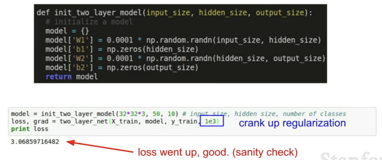
• crank up regularization, to see that loss goes up (b/c we added an additional regularization term)
  • sanity check

Step 4; Start training

Sanity checks

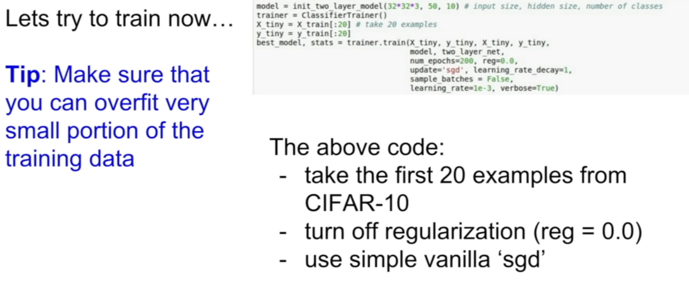
• good way to do this is to start up with a very small amount of data
  • should be able to overfit this very well and get very good training loss
• in this case, turn off regularization and see if we can make the loss go down to 0

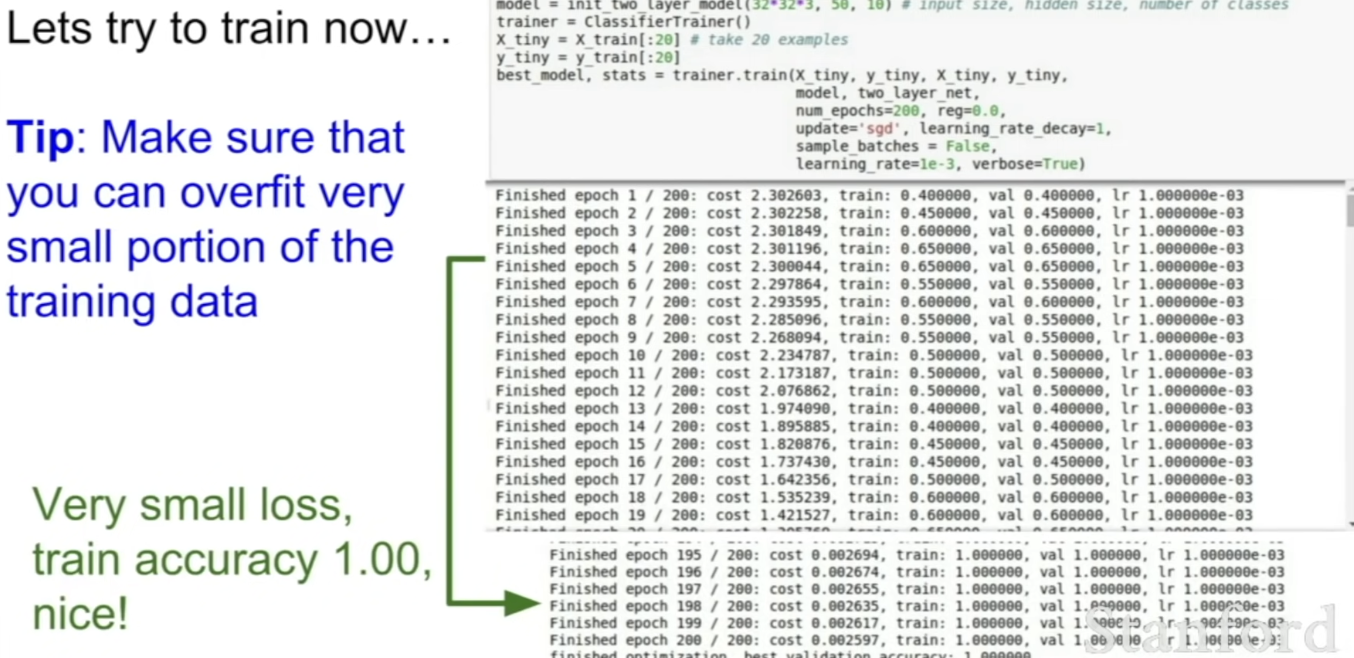
• compute loss at each epoch, see this go all the way down to 0
• also training accuracy goes up to 1 = makes sense

Actual training

• start with a small amount of regularization and figure out what a good learning rate is
  • learning rate is a hyperparameter
• try some value of learning rate
  
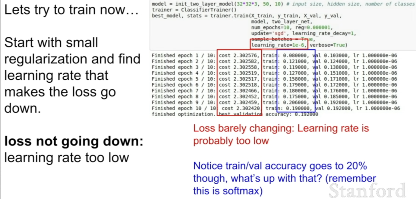
  - when learning rate is too small, gradient update is not big enough
  - but, training and validation accuracy jumped up to 20% very quickly
  - probabilites are still diffuse, so loss term is still similar
  - but when we shift all of these probabilities slightly in the right direction, now the accuracy all of a sudden jump b/c we're taking the maximum correct value
  
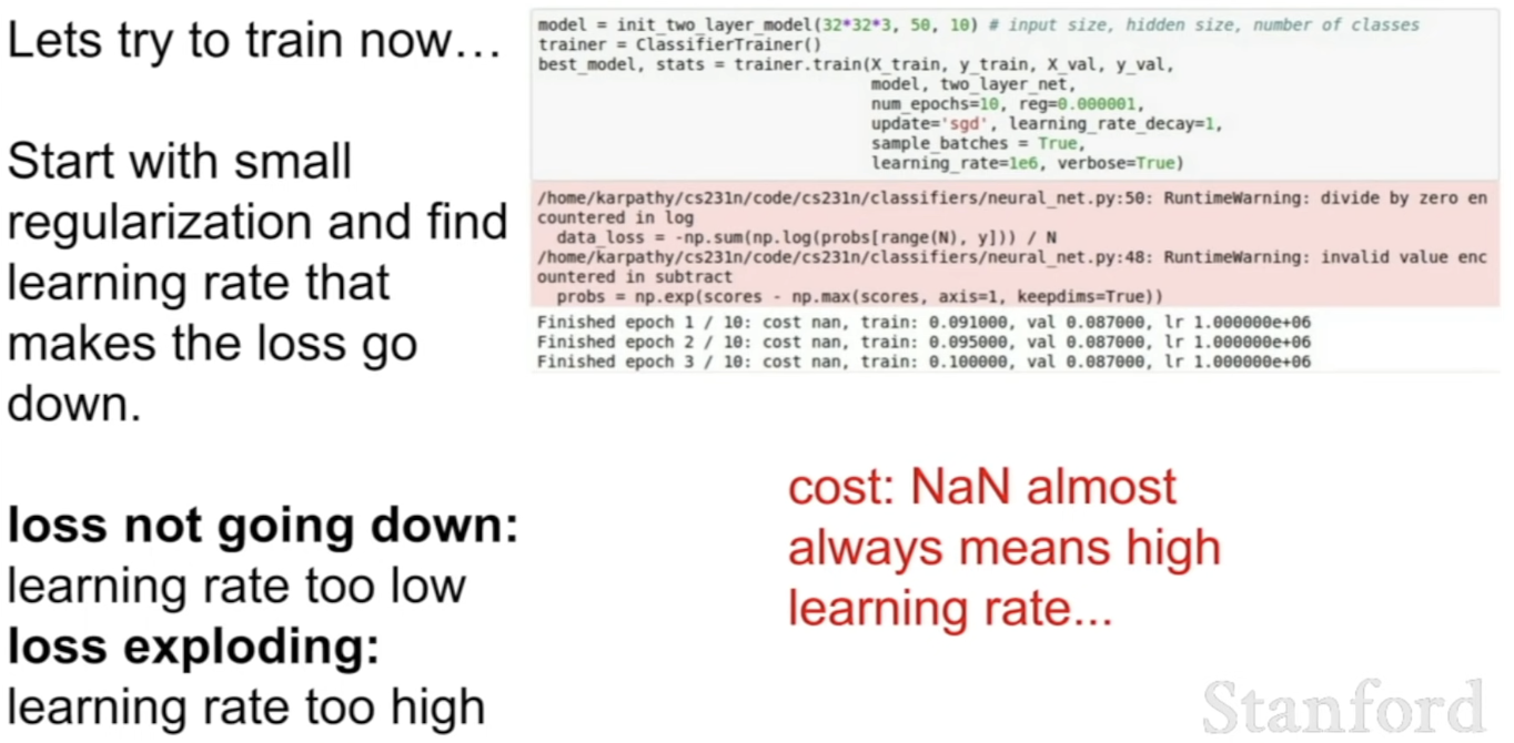
  - pick a very big learning rate, 1e6
  - cost is giving us NaN = cost exploded → b/c learning rate was too high
  
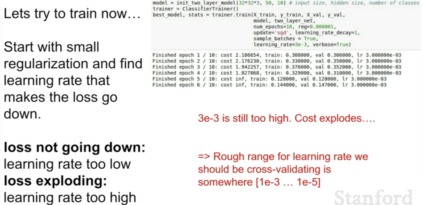
• try out values in this range, and depending on the loss, adjust it based on this

Hyperparameter Optimization

Cross-validation strategy

• for any hyperparameters

• training on the training set, evaluating on a validation set (how well this hyperparameter did)
  1. coarse stage
  - pick values spread out apart, learn for only a few epochs
  - can see what the good range is
  2. fine stage
  - run this for a longer time, and do a finer search over that region

• Tips for detecting explosions like NaN

  • in the training loop, sample some hyperparameter, start training, and look at the cost at every iteration or epoch
  • if cost > 3 * original cost ⇒ not heading in the right direction = break out, stop this hyperparameter choice

Example: 5 epochs

Coarse search

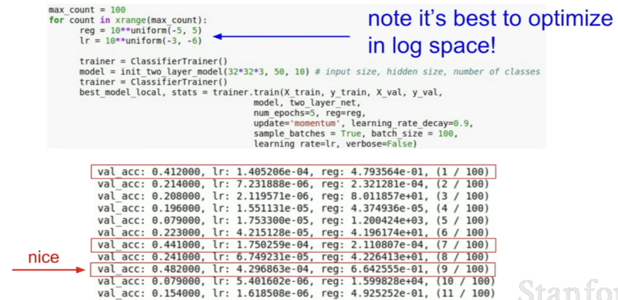
• red boxed are the regions that we'll look into more detail
• note: better to optimize in log space
  • instead of sampling between 1e-0.01 to 1e100
  • do 10 to the power of some range
  • b/c learning rate is multiplying the gradient update, it has multiplicative effects. so it makes more sense to consider a range of learning rates that are multiplied or divided by some value, rather than uniformly sampled

Finer search

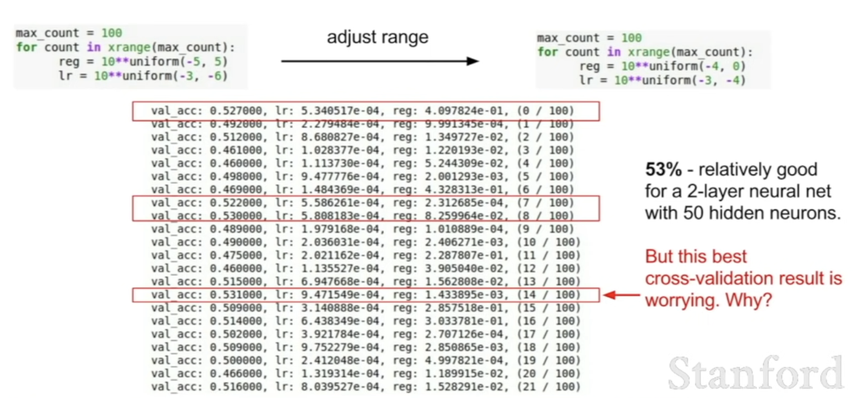
• now we have a range of $10^{-4}$, $10^0$
• we're getting a relatively good accuray of 53%, so this means that we're headed in the right direction
• problem: all of the good learning rates are at the edge of the range that we were sampling
  • bad
  • b/c this means that we might not have explored the space sufficiently
  • there might be better ranges if we continue shifting down
• make sure that range has the good values somewhere in the middle, so that the range was explored rangefully

Random search v. Grid search

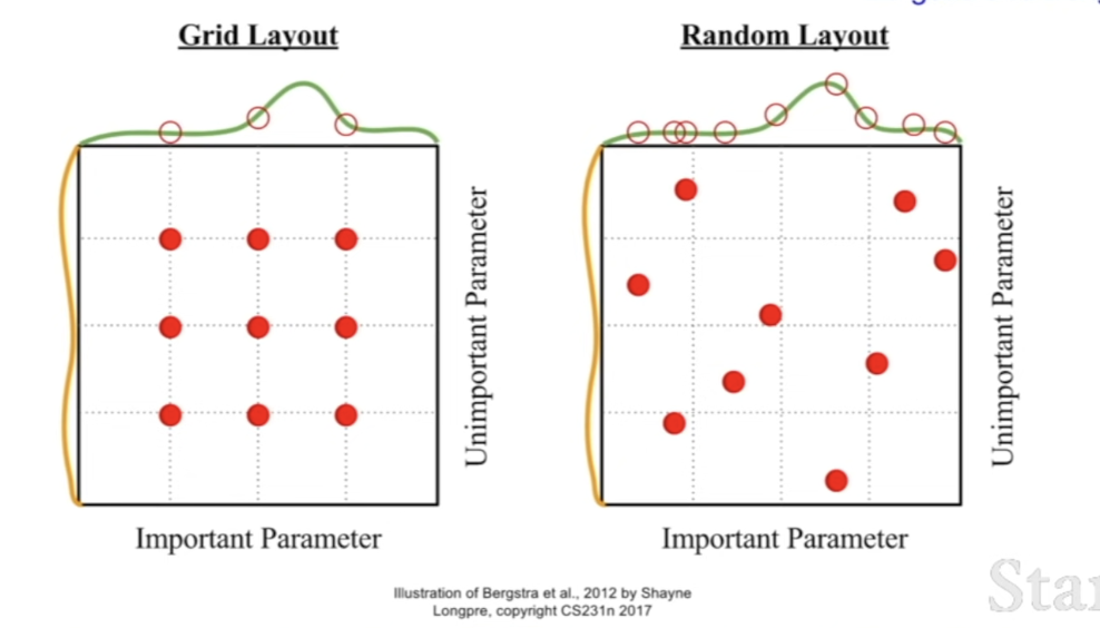
• we can sample different hyperparmeters using a grid search
  • fixed set of values for each hyperparameter, sample in a grid manner over all of these values
• in practice, it's better to sample randomly
  • if a function is more of a function of 1 variable than another, we'll get many more samples of the important variable that we have
  • we'll be able to see the green function on top showing where the good values are
  • compared to grid layout, where we can only do 3 samples, and we've missed where the good regions are

Hyperparameters

• learning rate, its decay schedule, update type
• network architecture
• regularization (L2/Dropout strength)

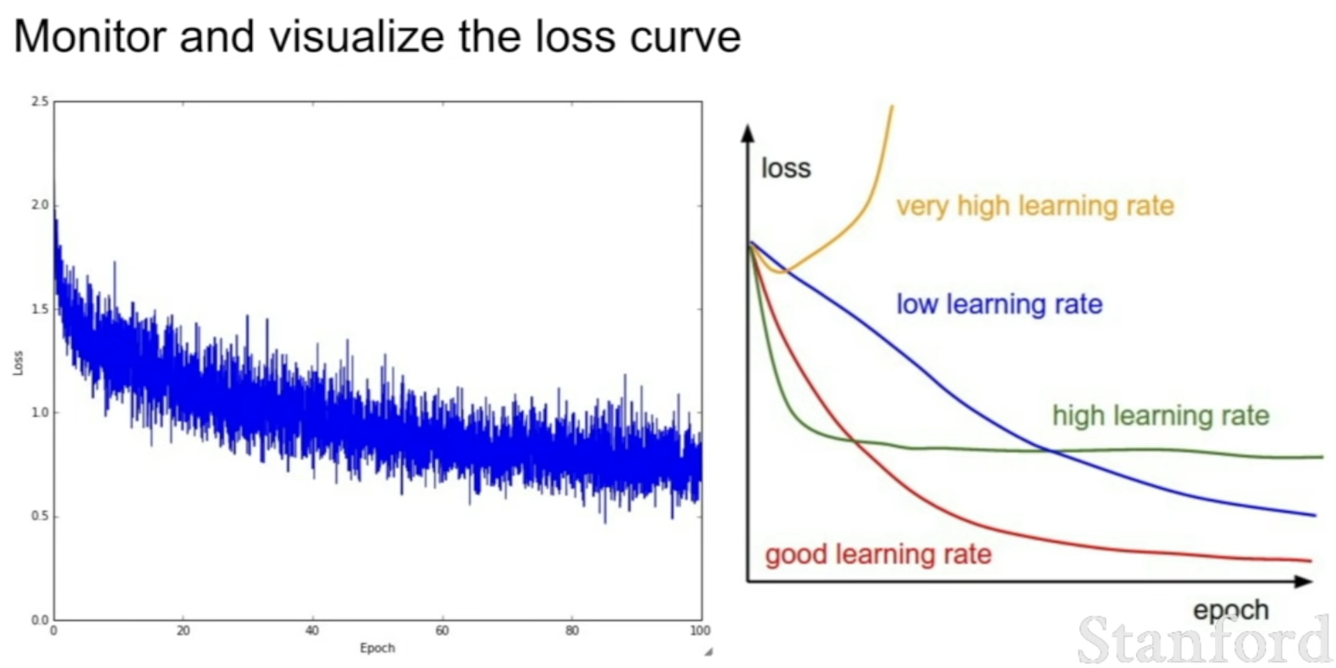
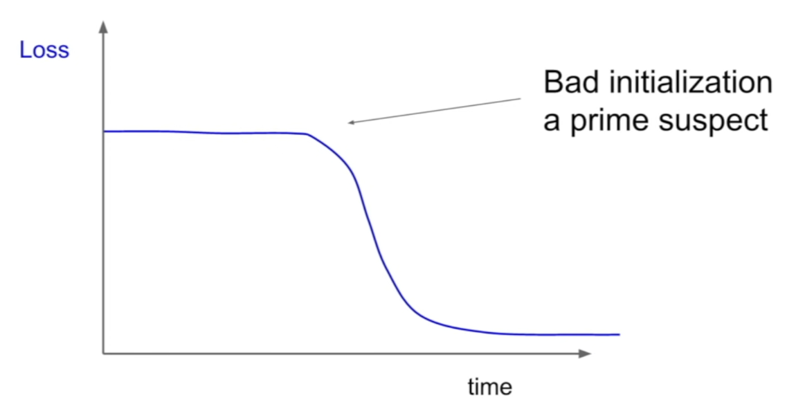
• potential reason = bad initialization
  • gradients are not really flowing too well at the beginning
  • so nothing's really learning
  • at some point, it just happens to adjust in the right way...

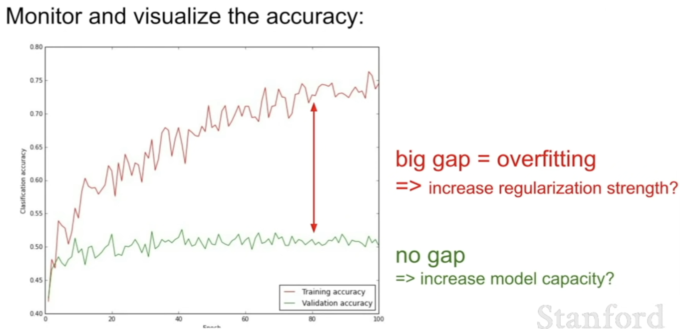
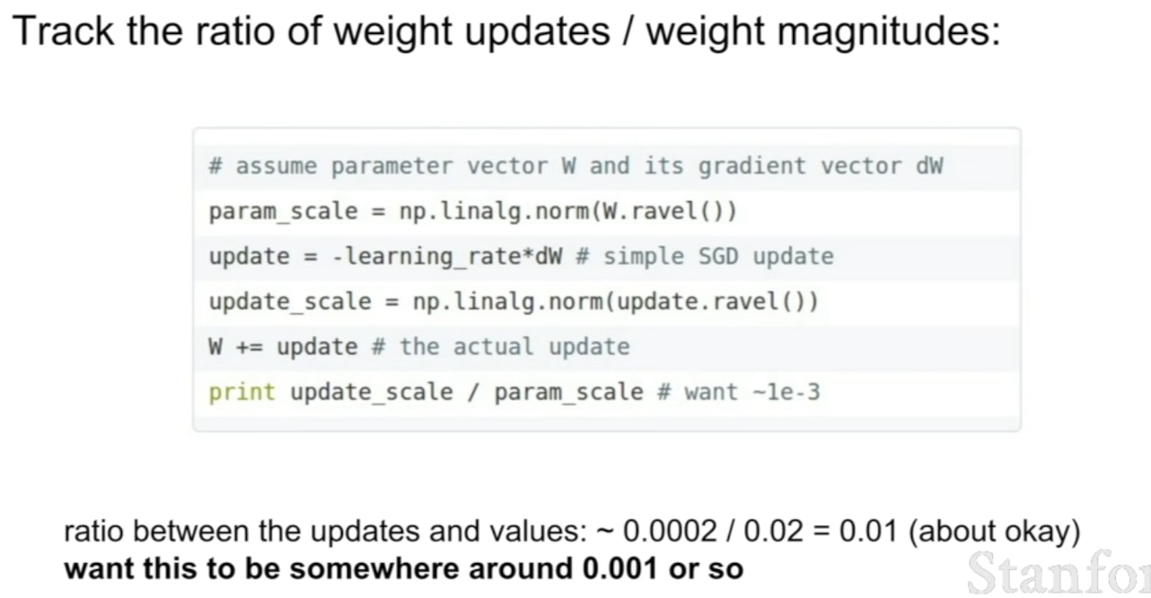
• track the update, the ratio of weight updates to the weight magnitudes
  • take the norm of parameter that we have to get a sense of how large they are
  • ratio to be somewhere around 0.001
  • just the sense that you don't want the updates to be too large compared to the value or too samll

Summary

• Activation Functions (use ReLU)
• Data Preprocessing (images: subtract mean)
• Weight Initialization (use Xavier init)
• Batch Normalization (use)
• Babysitting the Learning process
• Hyperparameter Optimization (random sample hyperparameters, in log space when appropriate)