🔎 Stanford CS231n 강의를 듣고 기록용도로 정리하는 게시글입니다.

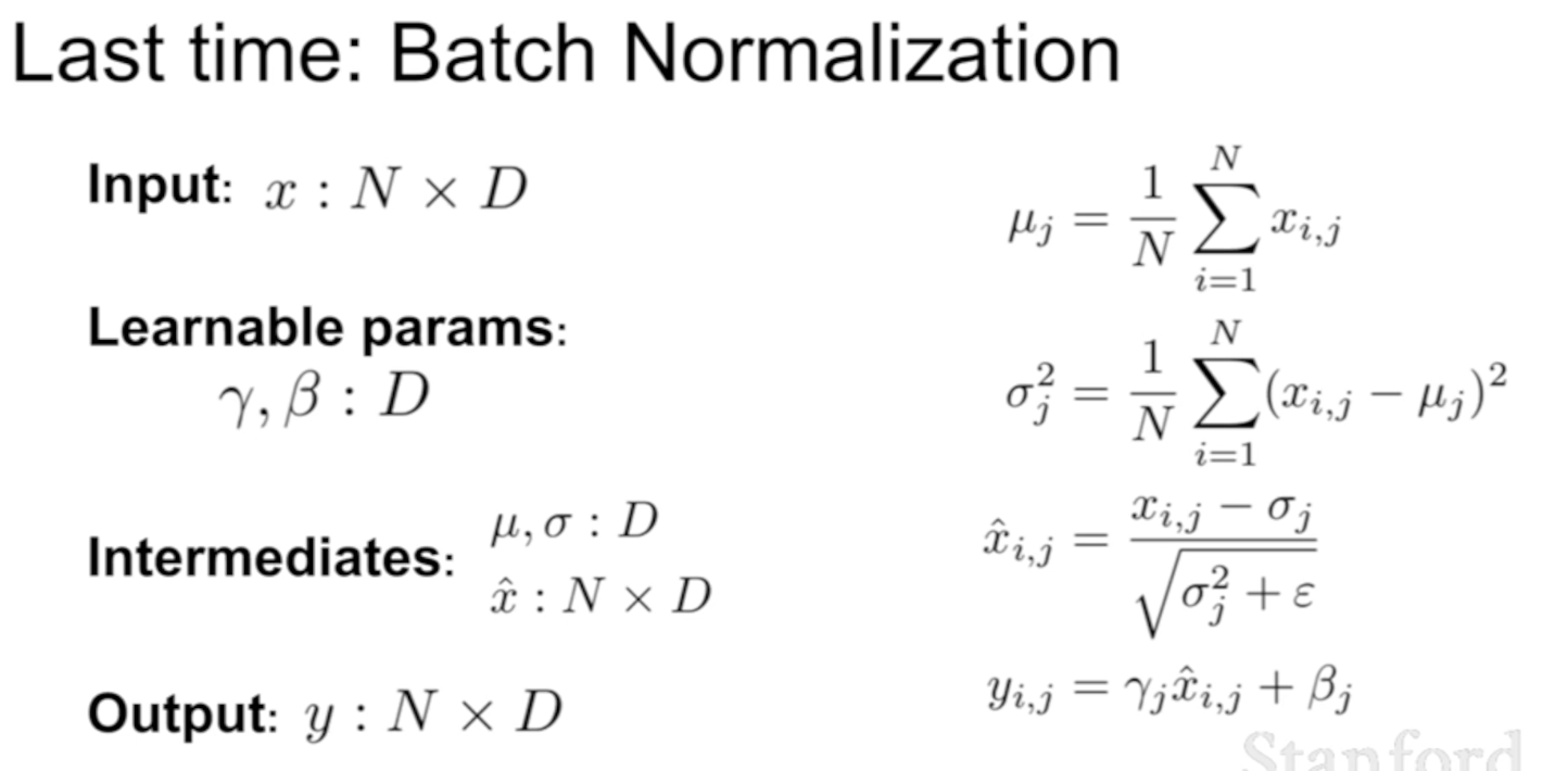
• add additional layer to force all intermediate activations to be zero mean and unit variance

Fancier Optimization

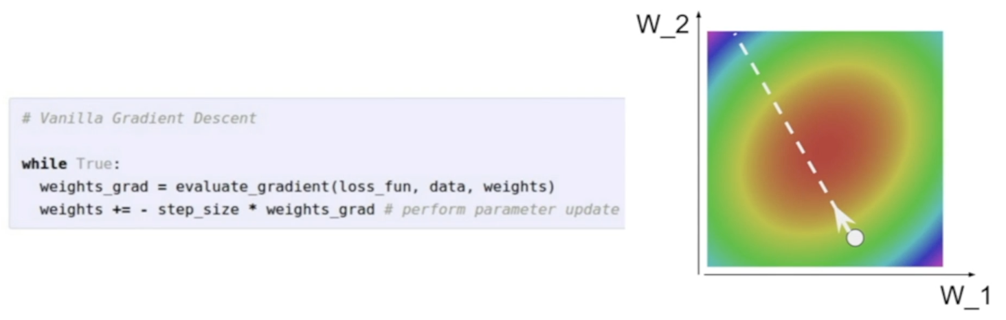
• core strategy in training neural networks: optimization problem
  • loss function defines for each value of the network weights, how good or bad is the value of weights doing on our problem
  • loss functions give us landscape over the weights

Problems with SGD

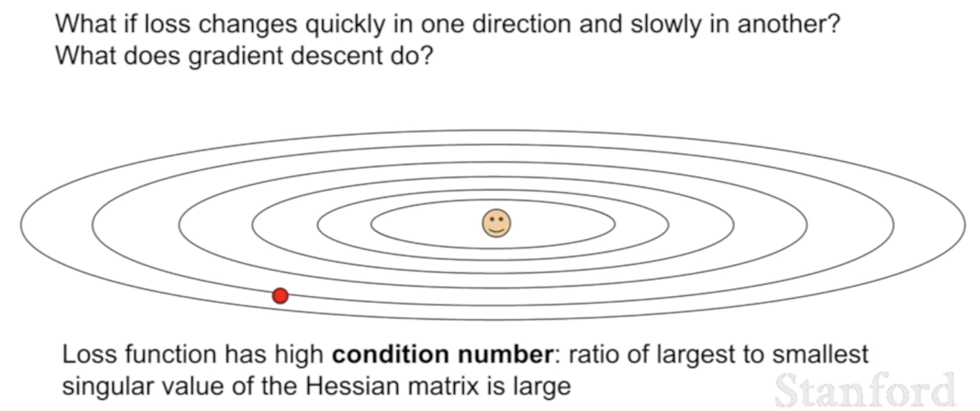
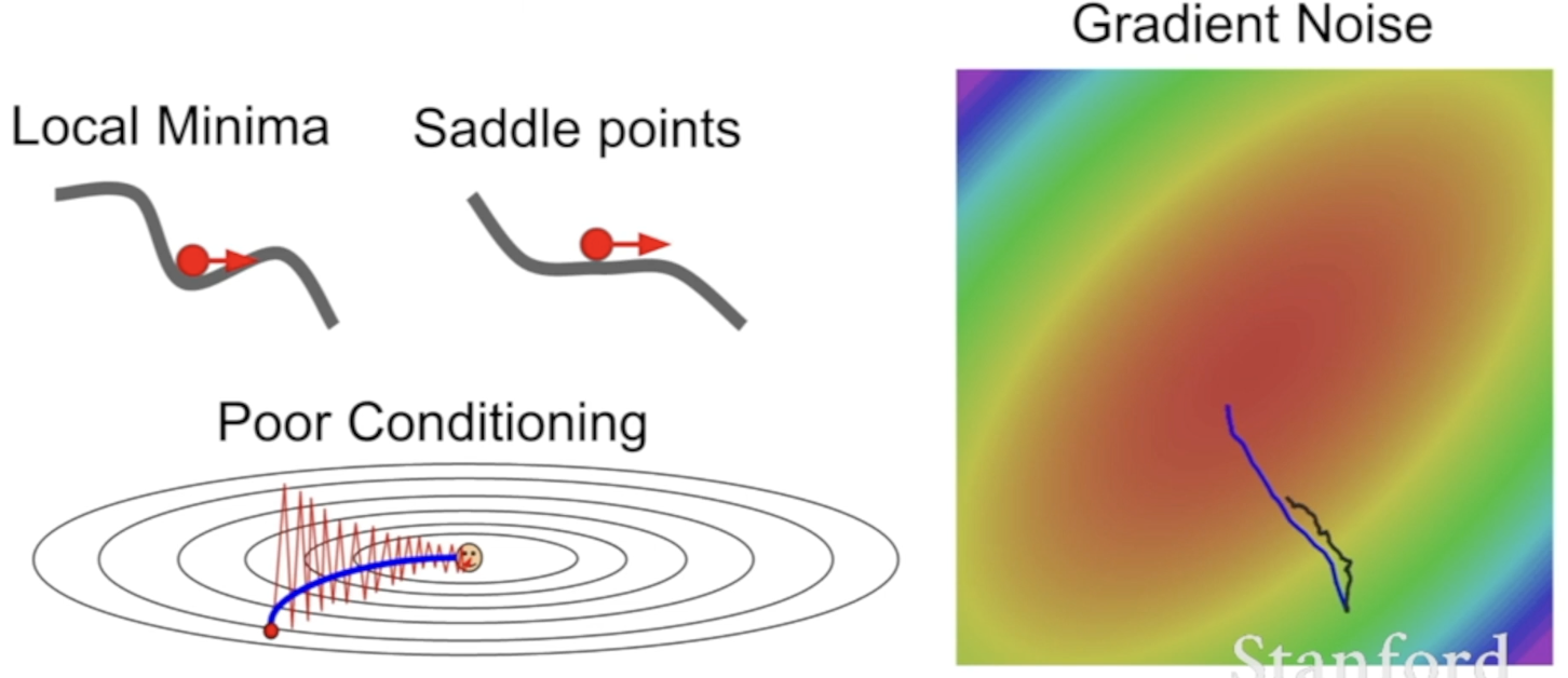
1. Say that we have 2 values($W1, W2$), and as we change of those values, the loss function changes very slowly

• In the picture, the loss is very sensitive to changes in vertical direction. (= like a taco shell)
• What might SGD do on a function that looks like this?
  
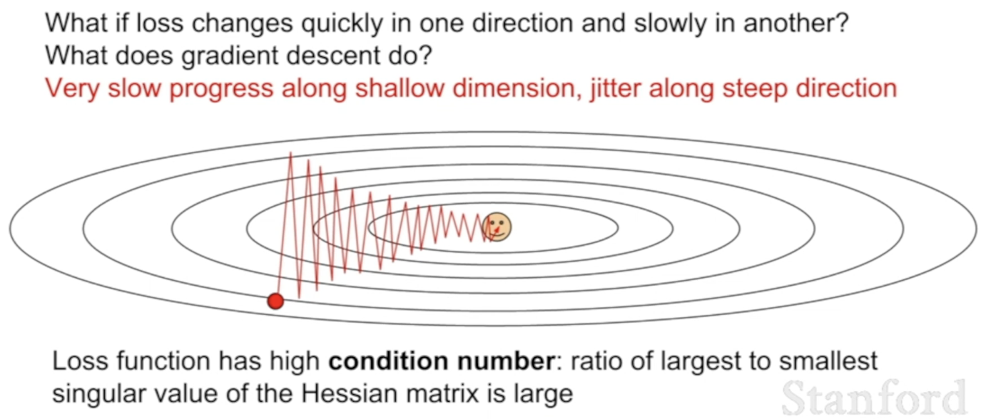
  • might get zigzagging behavior, b/c the direction of the gradient does not align with the direction towards the minima
  • very slow progress along the horizontal dimension and zigzagging, fast changing behavior across the fast-changing dimension (=undesirable)
    • this problem becomes much more common in a higher dimension
    • in practice, neural networks might have tens of millions of parameters = tens of millions of directions along which this thing can move. and if the ratio between the largest one and smallest one is bad = SGD will not perform nicely

2. Local minima & Saddle point

• What if the loss function has a local minima or saddle point?
  
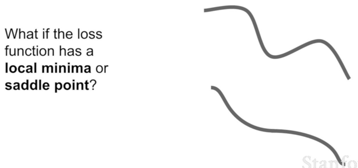
  • X axis: value of 1 parameter, Y axis: value of loss
    
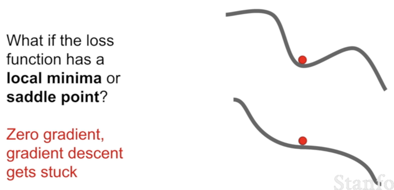
  • at the local minima, the gradient is 0 (b/c it's locally flat) → gets stuck
    • In SGD, compute the gradient and step in the direction of opposite gradient
  • Saddle point: A point where in one direction we go up, and in the other direction we go down
    • get stuck, b/c the gradient = 0
• In high dimension, saddle point means that at the current point, some directions, the loss goes up and some directions, loss goes down
  • saddle point will happen almost everywhere
    • region near saddle point is also a problem
    • here, gradient isn't 0 but slope is very small = we'll make very slow progress
  • whereas the local minima is saying that all of those 100 million directions I can move, every one of them causes the loss to go up (= pretty rare
  • so, when training large neural networks, the problem is saddle points >>> local minima

3. Being stochastic
   

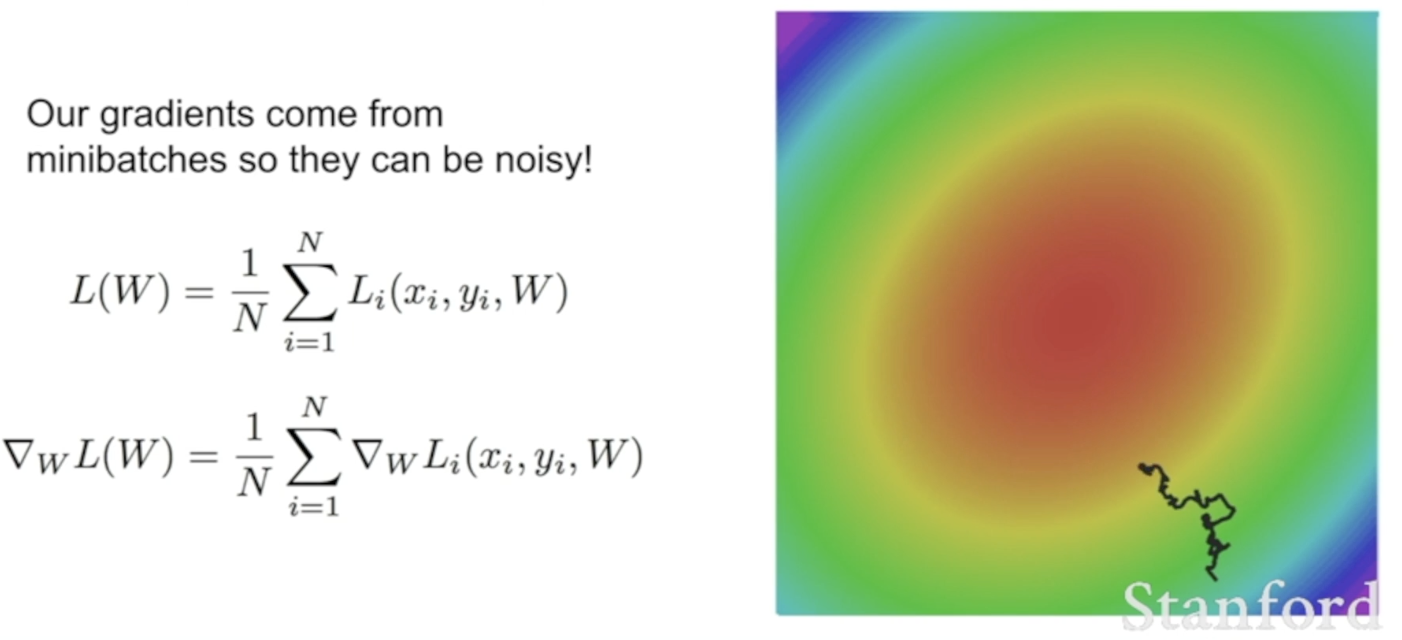
• We estimate the loss and the gradient from small mini batch of examples
  • Meaning that we're not getting a true information about the gradient at every time step
  • Instead, we're getting a noisy estimate of the gradient at our current point

SGD + Momentum

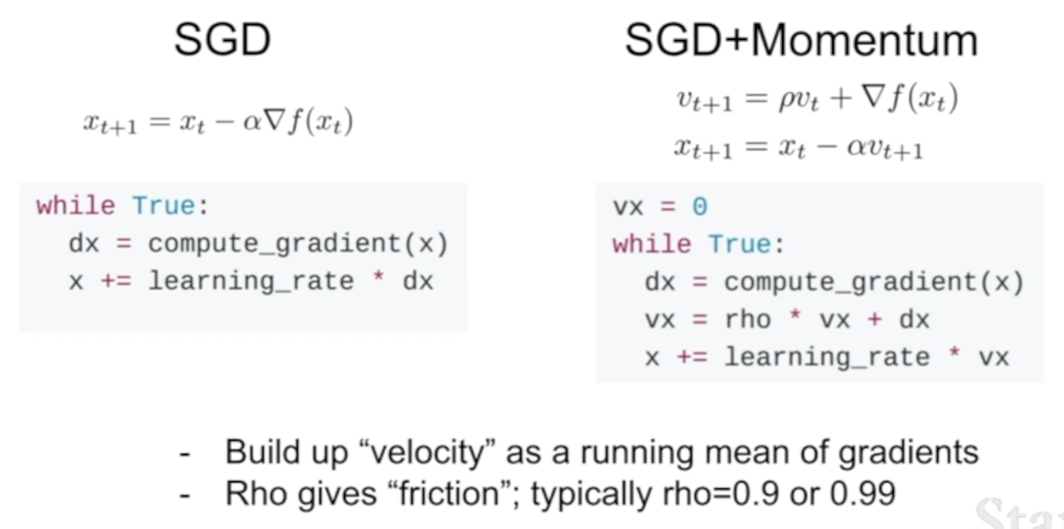
• maintain the velocity over time, and add gradient estimates to the velocity → step in the direction of the velocity (rather than in the direction of the gradient)
  • velocity init: 0
• hyperparameter $\rho$ corresponds to friction
  • at every time step, decay the current velocity by the friction constant $\rho$ (a high value ex.0.9), add in the gradient, step in the direction of velocity vector

• black line: vanilla SGD / blue line: SGD + momentum

• Considering velocity in this system, we can have a physical interpretation of this ball rolling down the hill and picking up speed as it comes down

• once we have velocity, even when we pass the point of local minima, point will still have velocity even if it doesn't have gradient ⇒ can get over the local minima and continue downward

• Gradient around saddle point is very small, but we have velocity vector as we roll down hill → can carry us through the saddle point and let us continue rolling down

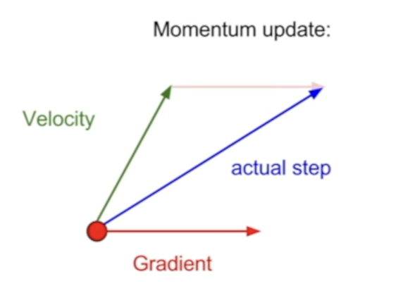
• red: current point, red vector: direction of the gradient (or estimate of the gradient)
• green: direction of velocity vector
• when doing momentum update - stepping according to weighted average of the red and green
  • helps overcome the noise in the gradient estimate

Nesterov Momentum

• variation of momentum
• start at the red point, step in the direction of where the velocity would take you, evaluate the gradient at that point, go back to the original point, and mix together those two

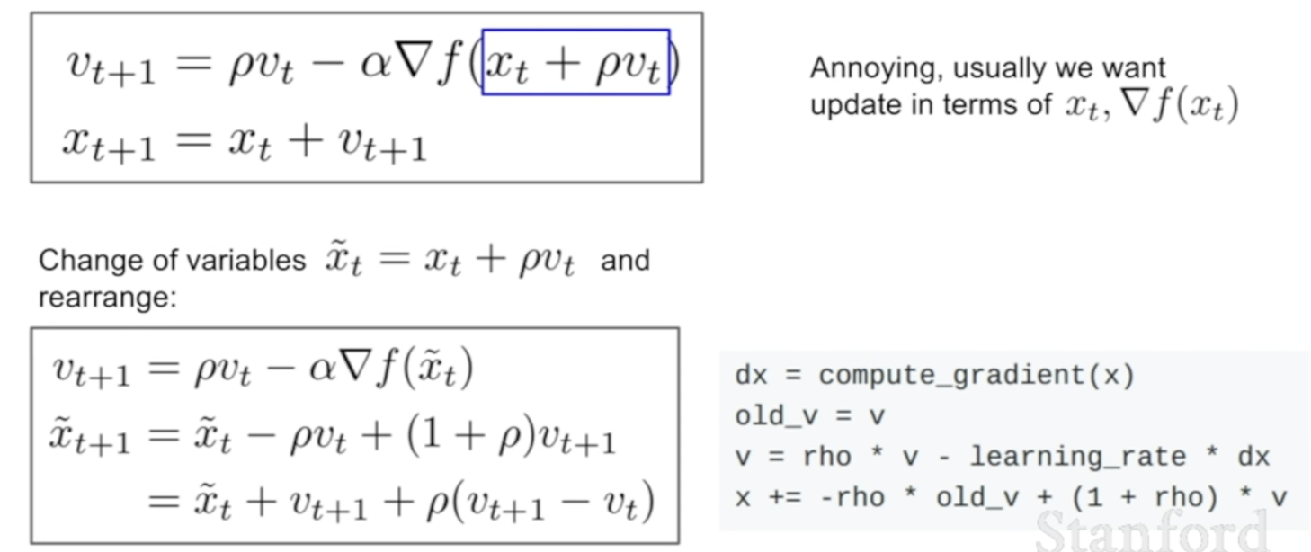
• to update velocity,
  • take a step according to previous velocity and evaluate the gradient there
  • take a step in the direction of velocity that's incorporating information from these multiple points

AdaGrad

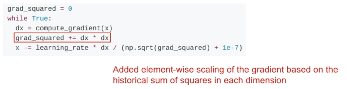
• during the course of the optimization, keep a running estimate or a running sum of all the squared gradients that you see during training
  • during training, keep adding the squared gradients to this grad squared term
  • when updating parameter vector, divide by grad squared term

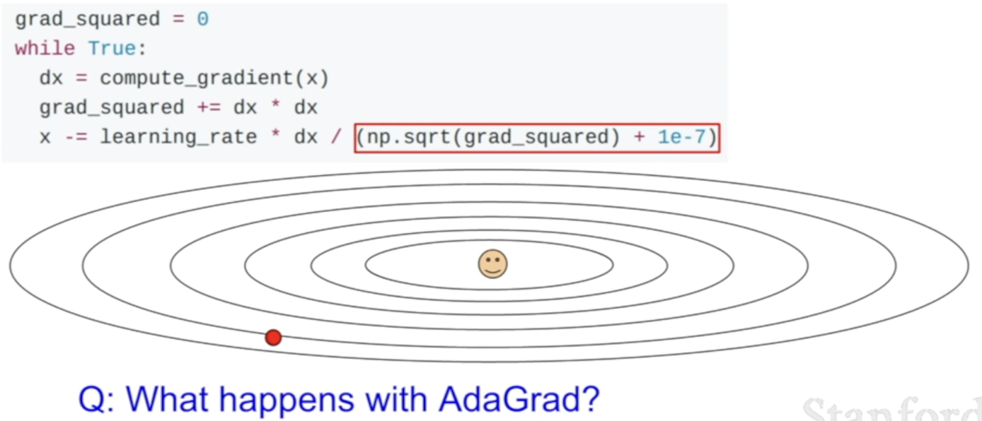
• What does this kind of scaling do where we have a very high condition number?
  • If we have 2 coordinates, one that always has a very high gradient and one that always has a small gradient, as we add sum of the squares of the small gradient, it means that we're diving by a small number, so we'll accelerate movement along the one dimension,
  • and along the other dimension where the gradients tend to be large, we'll be dividing by a large number, so we'll slow down the progress
• What happens to the step size over long time?
  • With AdaGrad, steps get smaller and smaller, b/c since we continue updating the estimate of the squared gradients over time, this estimate will grow, causing the step size to get smaller
  • This is actually good in convex(볼록한) case
    • b/c as you reach the minimum, you want to slow down to converge
  • In non-convex case, this is problematic
    • b/c as you come downwards the saddle point, might get stuck with AdaGrad and no longer make any progress

RMSProp

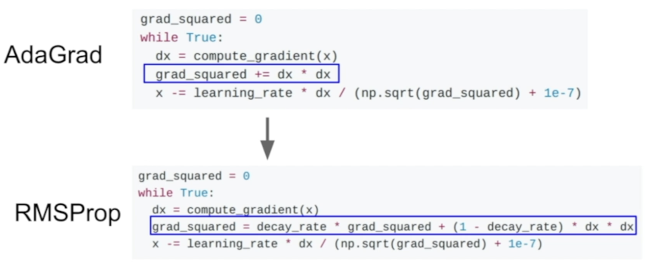
• variation of AdaGrad
• still keep the estimate of squared gradients, but instead of accumulating it over training, let that squared estimate decay
  • after computing gradient,
  • take current estimate of the grad squared, multiply it by decay rate(commonly .9 or .99)
  • add (1-decay_rate)*dx^2
  • step is exactly the same as AdaGrad, dividing by the squared gradient

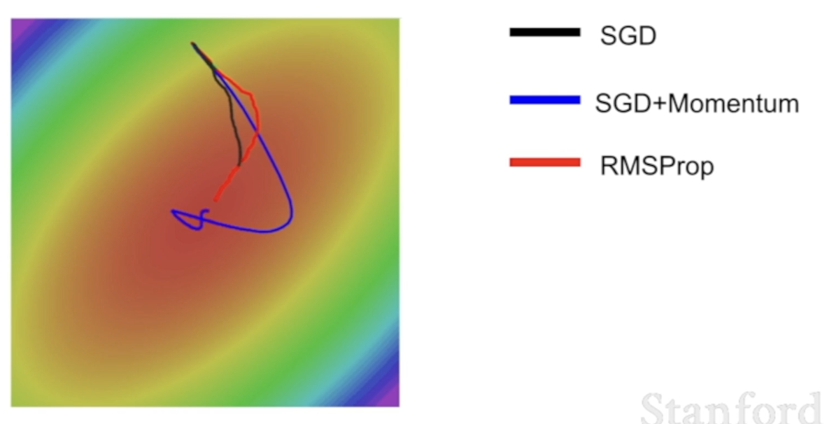
• RMSProp and Momentum are both doing better than SGD but their qualitative behavior is bit different
  • With SGD+Momentum, it overshoots the minimum and comes back
  • RMSProp is adjusting its trajectory(궤도) approximately equal to progress among all the dimensions

Adam (Almost)

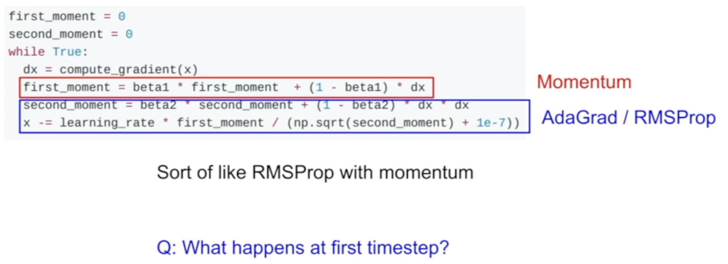
• maintain the estimate of the first moment and second moment
• red: make estimate of the first moment as a weighted sum of gradients
• blue: moving estimate of the squared gradients
• step using both the first moment (= velocity), divide by the second moment(=squared gradient term)
• What happens at first timestep?
  • at the beginning, initialized second moment with 0
  • beta2, second moment decay rate is 0.9 or 0.99
  • after one update, second moment is still very very close to 0
  • and when making a step, we're dividing by a very small number, so it's taking a very large step at the beginning

Q: What is the 1e-7 term?
A: to make sure we're not dividing by zero, adding a small positive number

Adam (Full form)

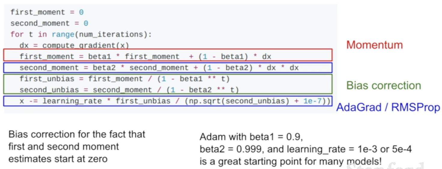
• with Adam above, in the first couple step, we might take a very large steps and mess up
• So, Adam adds bias correction term to avoid the problem of taking very large steps at the beginning
  • after updating first and second moment, we create an unbiased estimate of the first and second moments by incorporating the current time step (t)
  • now make a step using unbiased estimates, rather than the original first and second moments

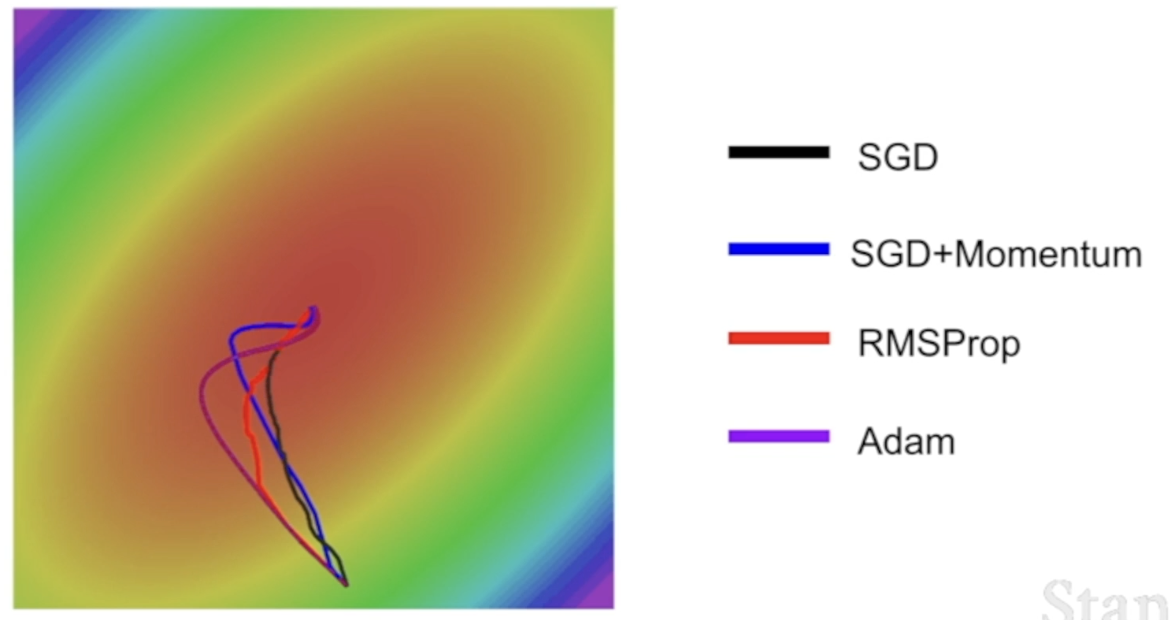
• Adam overshoots the minimum like SGD + momentum, but it doesn't overshoot as much as SGD + momentum
• Adam has this behavior of RMSprop of trying to curve, to make equal progress along all dimensions
• kind of combining the behaviors of both momentum and RMSProp

About Learning rate

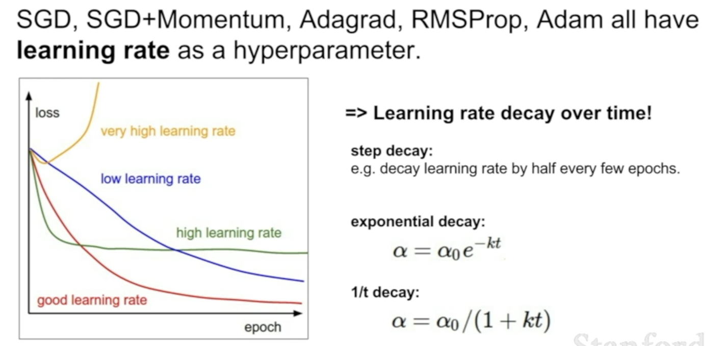
• It's tricky to pick the right learning rate
• Decaying the learning rates over time
  • combine the effects of these different curves, get the nice properties each

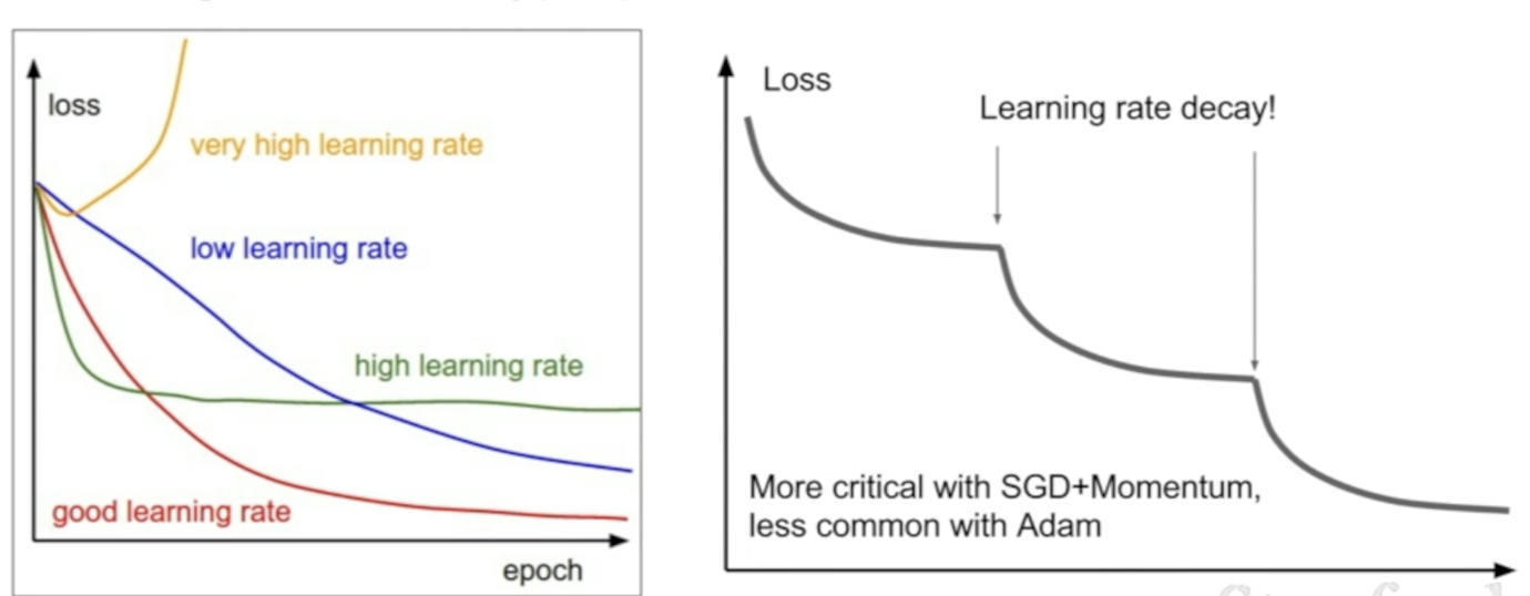
• using step decay learning rate

• learning rate decay is more common with SGD+Momentum, but less common with Adam

• learning rate decay is second-order hyperparameter

  • you should not optimize this from the start
  • when getting networks to work at the beginning, you want to pick a good learning rate with no learning rate decay from the start
  • so, try with no decay and see what happens, and see the loss curve and see where you think you might need decay(다른 값들이랑 동시에 최적화하려고 하면 헷갈리기만 함)

First-Order Optimization

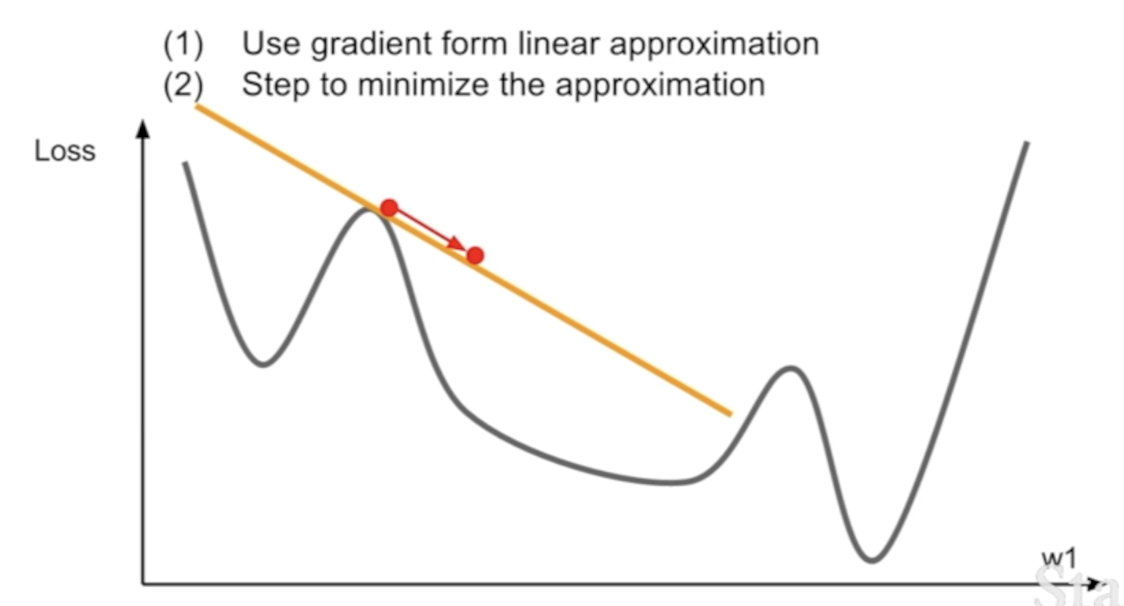
• we're computing the gradient at the current point (Red point)
  • using gradient information to compute linear approximation to our function (= First-order Taylor approximation)
  • pretend the first-order approximation is actual function, and take a step(not too far) to minimize the approximation
  • here, we're only incorporating information about the first derivative of the function

Second-Order Optimization

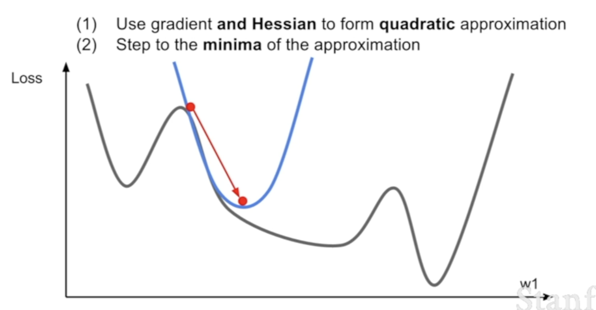
• take into account both the first and second derivative information
• make a second-order approximation to the function, locally approximate our function with quadratic

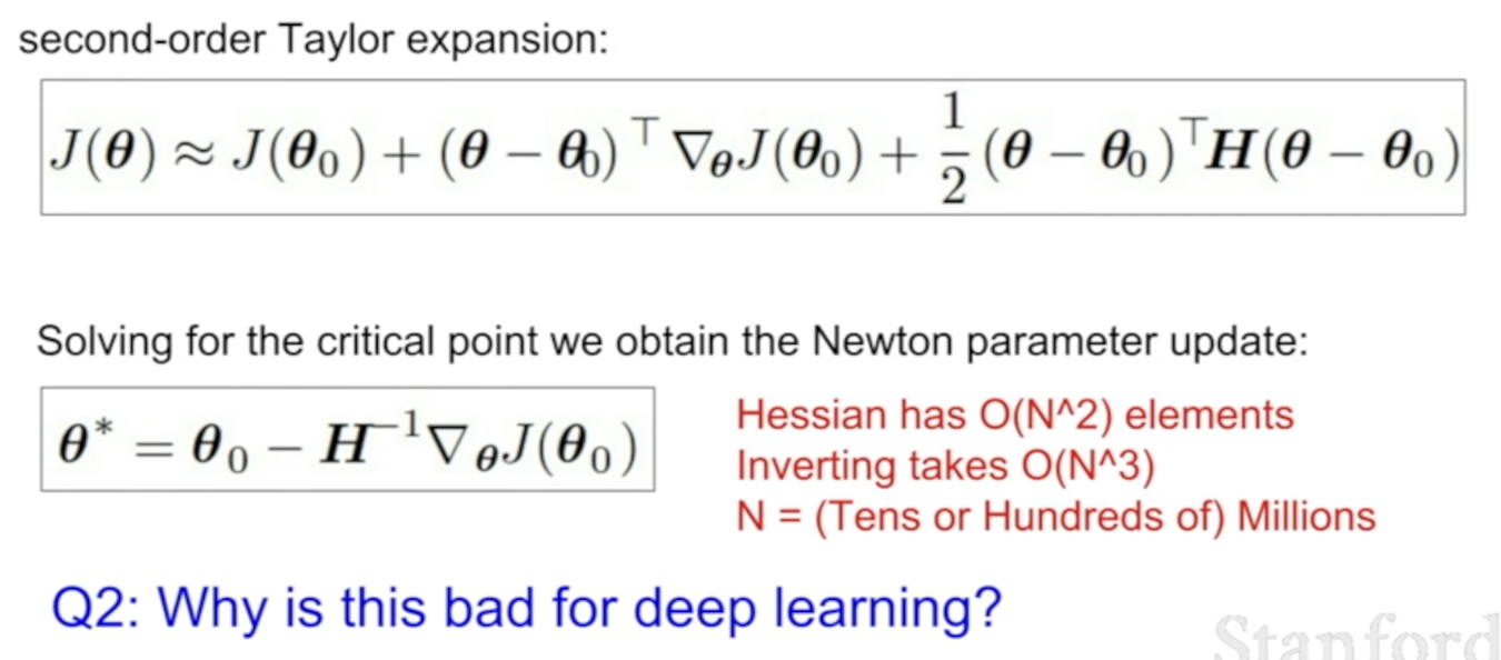
• generalizing this to multiple dimensions = Newton Step
  • compute Hessian matrix (matrix of second derivatives = 이계도함수(미분 두 번 한 것))
  • inverting this matrix in order to step directly to the minimum of this quadratic approximation to your function
• IT DOESN'T HAVE LEARNING RATE
  • here, we're making quadratic approximation and stepping right to the minimum of the quadratic
• However, bit impractical in practice
  • Hessian Matrix is NxN, where N is the number of parameters
  • If N = 100 milllion → 100 million squared is way too big, can't store that in memory and can't invert it

In practice

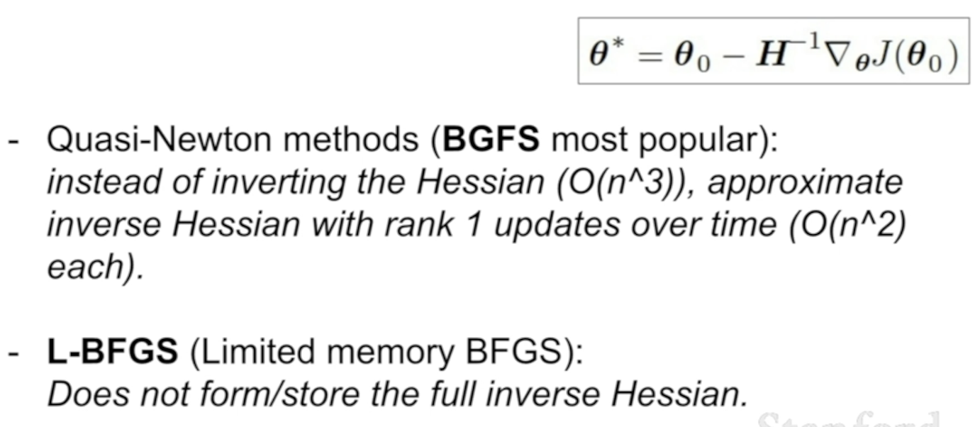
• rather than working with the full Hessian and inverting the full Hessian, work with approximations
  • low rank(행렬의 열 개수) approximations are common

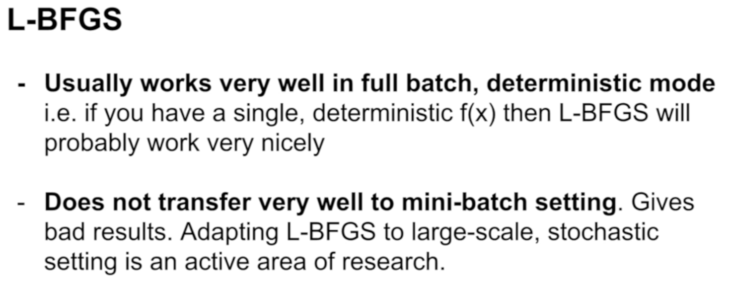
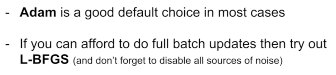
• keeps the approximation of the Hessian
• in practice, doesn't work too well
  • b/c they don't really handle the stochastic case very much
  • tend not to work so well with non-convex problems

Regularization

• all of these optimization algorithm is about reducing training error

• BUT we don't care about training error that much

• INSTEAD, we care about the performance on unseen data, care about reducing the gap between training and test error

• What can we do to reduce this gap?
  ⇒ a quick, easy but dirty thing to try = model ensembles

• rather than having just 1 model, train 10 different models independently from different initial random restarts

• at test time, run data through all 10 models and average the predictions of 10 models

• tends to reduce overfitting a little bit and improve performance a little bit, typically by a couple percent (not a drastic improvement)
  

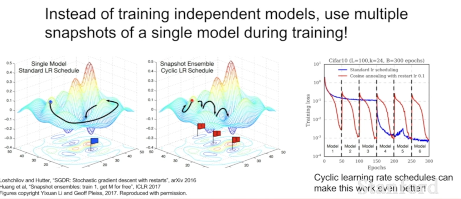
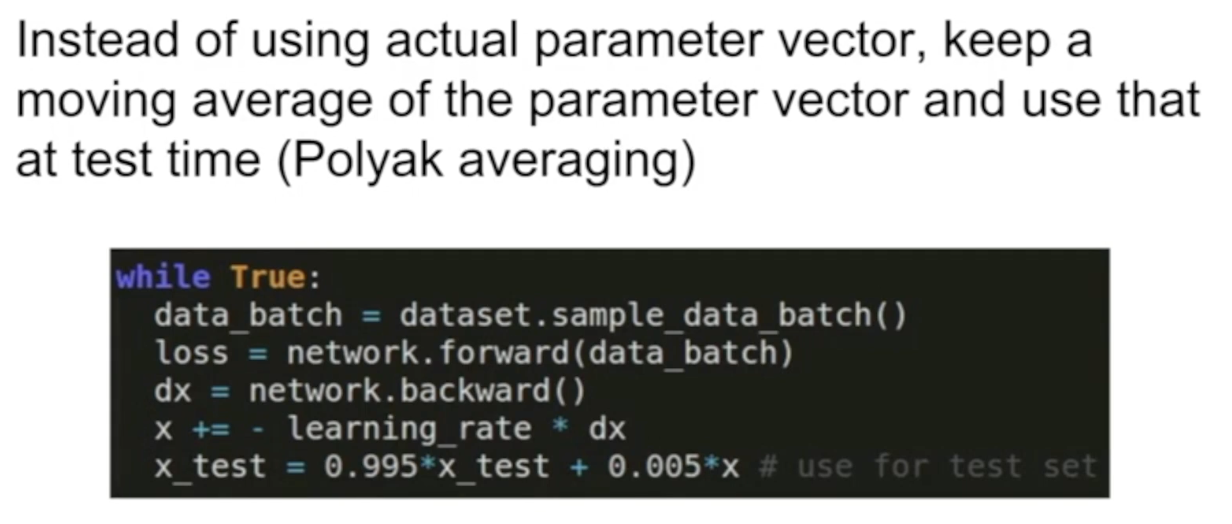
• during training, keep an exponentially decaying average of your parameter vector itself to have a smooth ensemble of your own network during training

---

• How to improve single-model performance? = Regularization
  - When we have ensembles, we have to run 10 models at test time -> not so great
  

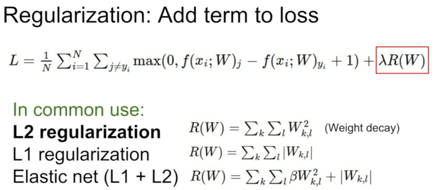
• adding explicit extra term to loss
  • BUT L2 regularization doesn't make a lot of sense in the context of neural networks

Dropout

• very common for neural networks
• every time when we do forward pass, at every layer, randomly set different subsets of neurons to 0 (1 layer at a time)
  • run through the layer → compute the value of the layer → randomly set some of them to 0 → continue

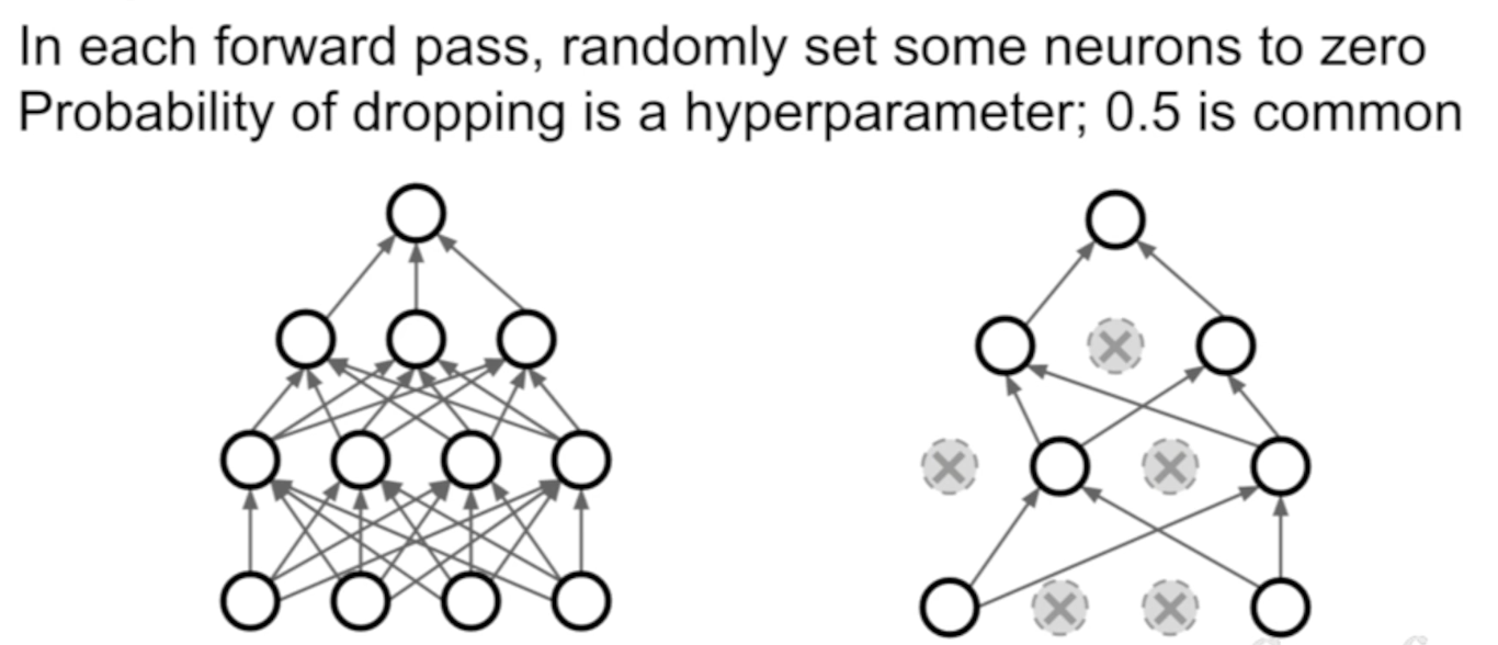
• left: fully connected layer / right: dropout version of the same network
• after we dropout, it looks like smaller version of the same network
  • the subset that we use varies at each iteration (at each forward pass)

Q: What are we setting to 0?
A: Activations. Each layer is computing $\text{previous activation} \times W = \text{next activation}$. Take that activation, set some of them to 0.

Q: At which layer do we do this?
A: Commonly on fully connected layers, but sometimes in convolutional layers

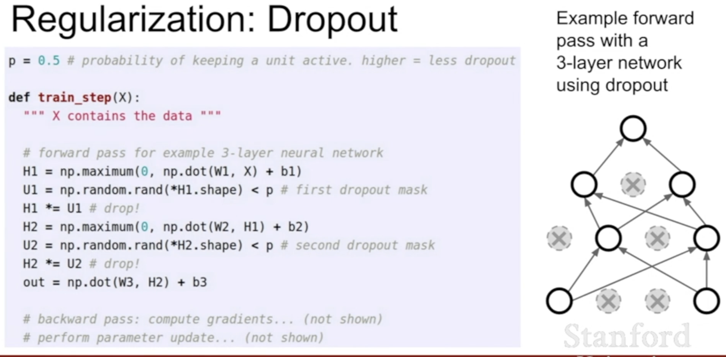
• 3-layer neural network

Why is this a good idea?

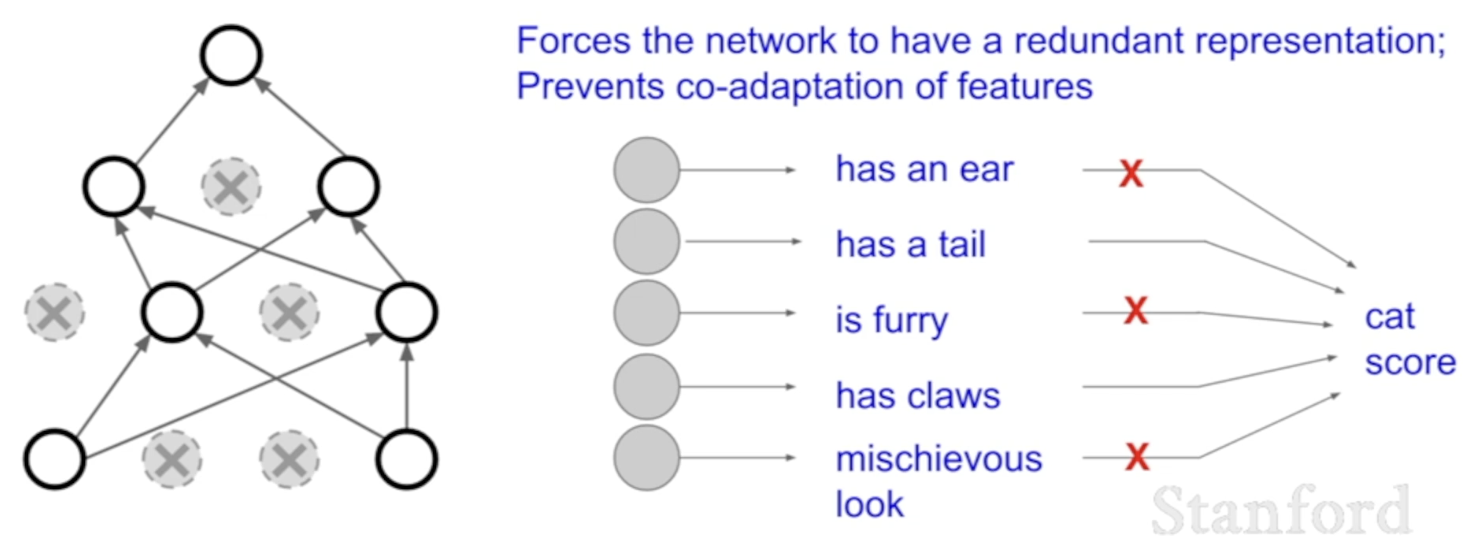
1. helps prevent co-adaptation of features
   • ex) when classifying cats, maybe in some universe, the network might have 1 neuron for having an ear, 1 neuron for having a tail ... and combine these things together to decide whether or not it's a cat
   • but using dropout, in making the final decision about catness, the network cannot depend too much on any of these 1 features
   • Instead, it needs to distribute its idea of catness across many different features ⇒ might help prevent overfitting somehow

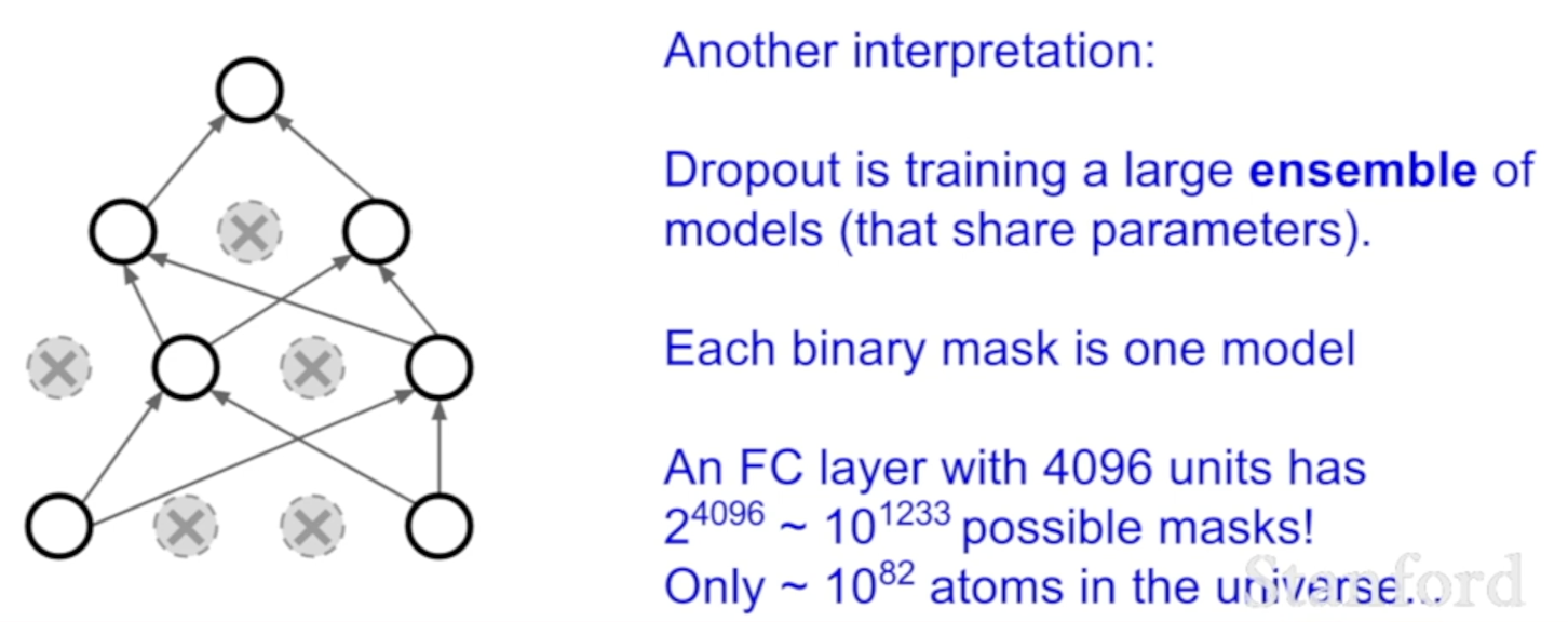
2. similar to doing model ensembling within a single model
   • after applying dropout, it's similar to computing this sub-network using some subset of the neurons
   • every different potential dropout mask leads to a different potential subnetwork → dropout is learning a whole ensemble of networks all at the same time that all share parameters
   • b/c the number of potential dropout masks grows exponentially in the number of neurons, you're never going to sample all of these things

At test time?

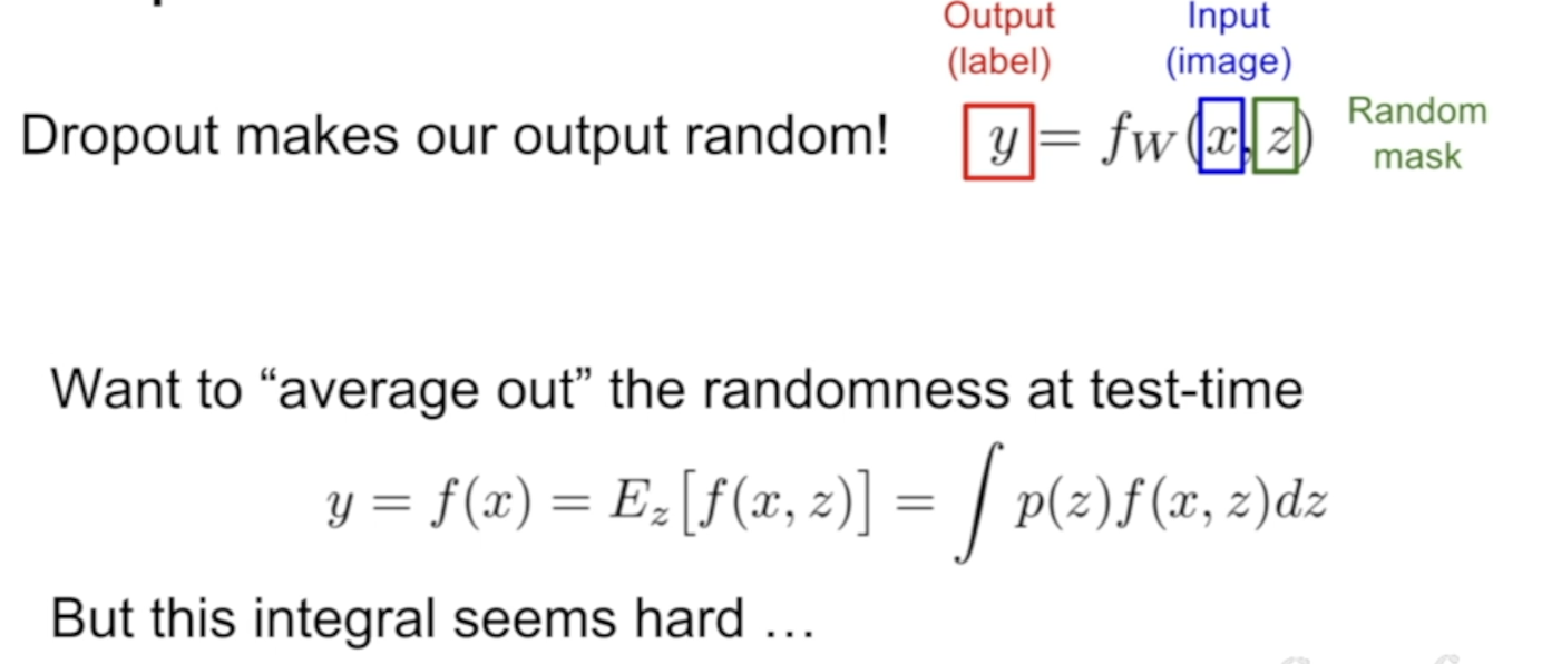
• fundamentally changed the operation of our neural network
• now, the network is also taking additional input $z$ (random dropout mask)
  • having randomness at test time is maybe bad
  • might want to eliminate this stochasticity at test time once the network is already trained
• then average out the randomness
  • you can marginalize out this randomness with integral
    • but this integral is intractable (아주 다루기 힘든)
  • can do approximating this integral via sampling, where you draw multiple samples of $z$ and average them out at test time
    • but still introduces some randomness, which is bad
• BUT we can approximate this integral in a cheap way locally
  • Consider a single neuron, output is $a$, inputs are $x, y$ with weights $W1, W2$
  • at test time, $a = w_1x+w_2y$
  • but during training, we use dropout with probability 1/2 of dropping neurons
    • so, expected value of $a$ during training = can compute analytically
  • so there's gap between the average
  • at test time we don't have any stochasticity → instead, multiply this output by the dropout probability
    

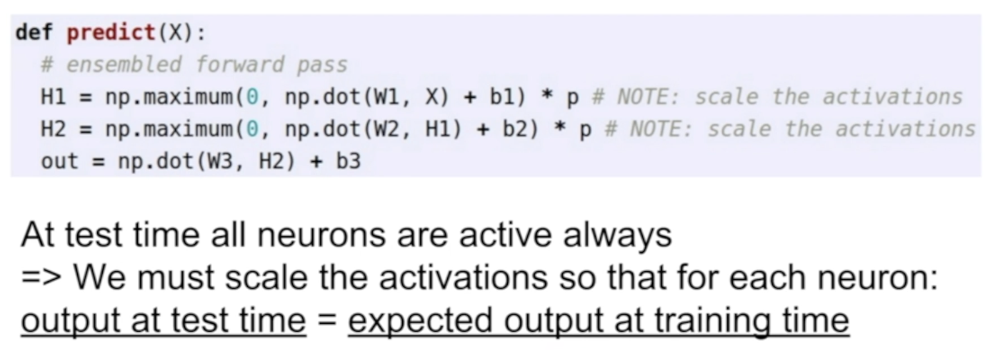
Dropout Summary

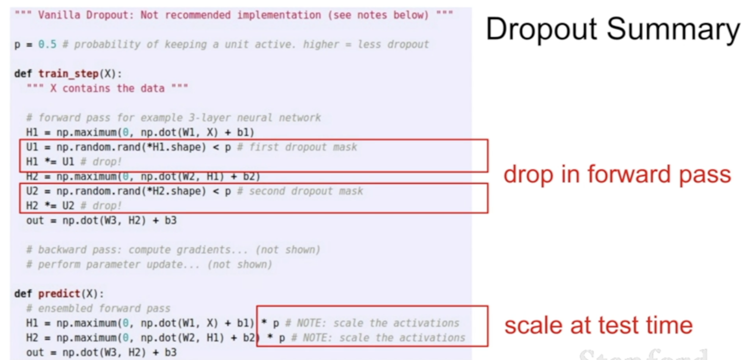
• randomly zero out some nodes
• at test time, in prediction function, add a multiplication by probability

Inverted Dropout

• more common
  
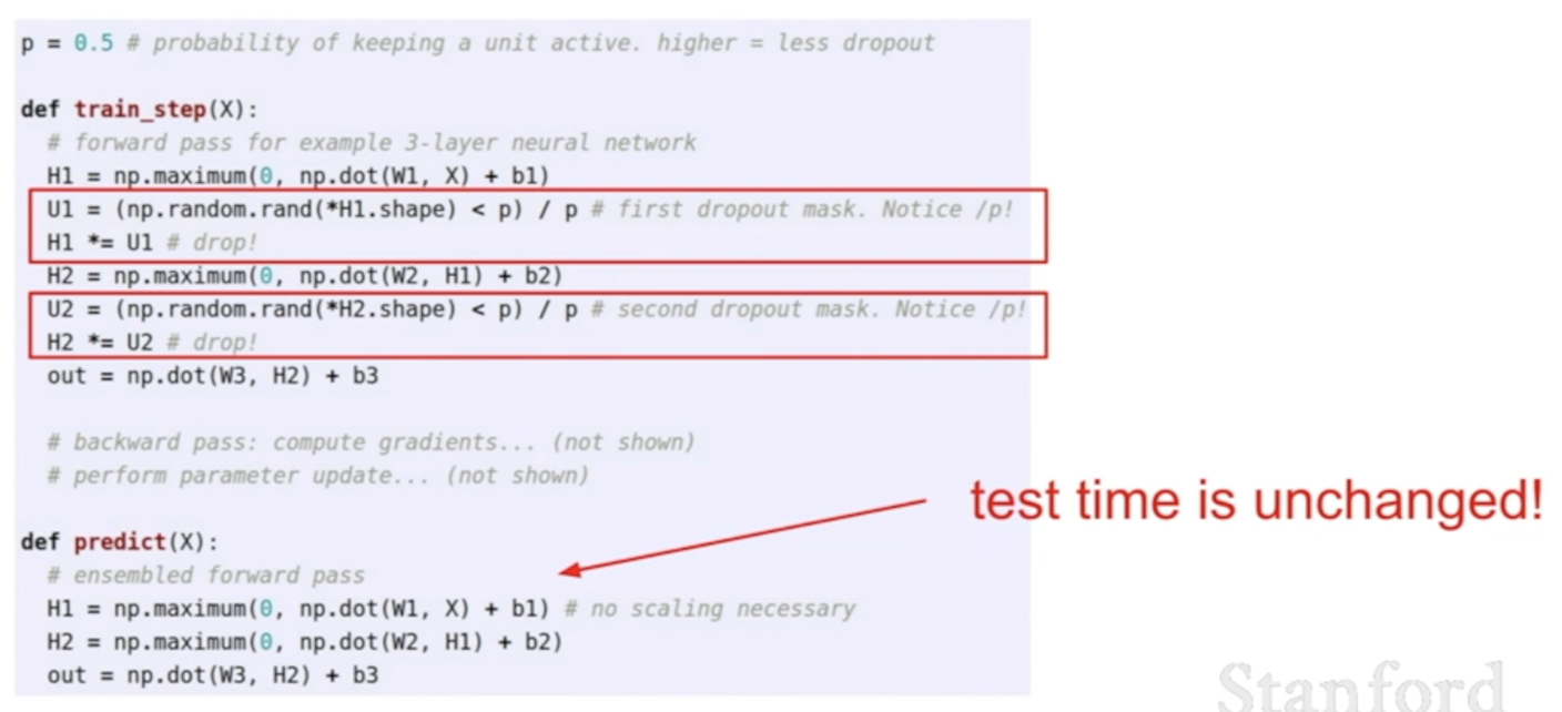
• at test time, you care more about efficiency → you want to eliminiate the multiplication of $p$
  • so at test time, use the entire $W$ matrix but at training time, divide by $p$

Q: What happens to gradient during training with dropout?
A: We end up only propagating the gradients through the nodes that were not dropped. This has the consequence that when you're training with dropout, training takes longer b/c at each step you're only updating some subparts of the network.

Common pattern

• general strategy for regularization
• When training, add some kind of randomness
  • to prevent it from overfitting
• When testing, average out all the randomness
  • to improve the generalization

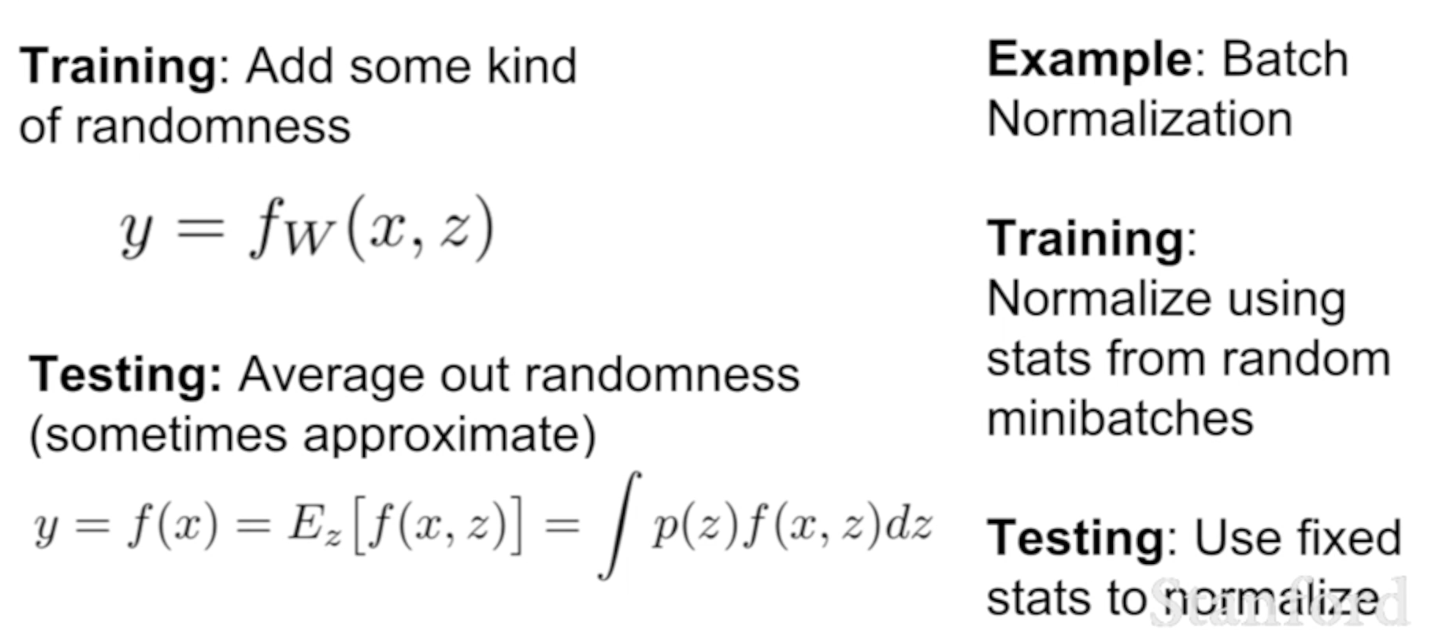
• Batch normalization fits this idea as well
  • during training, 1 data point might appear in different mini-batches with different other data points → still bit of stochasticity with respect to a single data point with how exactly that point gets normalized during training
  • during test time, we average out this stochasticity by using global estimates to normalize rather than the per mini-batch estimates
• when you train networks with batch normalization, sometimes you don't use dropout at all
• but dropout is nice b/c you can tune the regularization strength by varying the parameter $p$

Data augmentation

• during training, we can randomly transform the image in some way such that the label is preserved

Random crops and scales

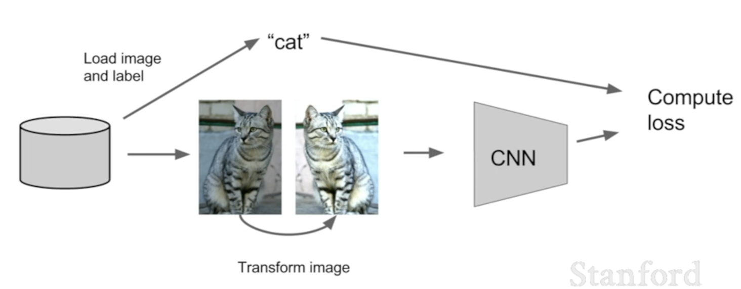
• flip horizontally, randomly crop or scale the image
• and train on these random transformations of the image rather than the original images
  
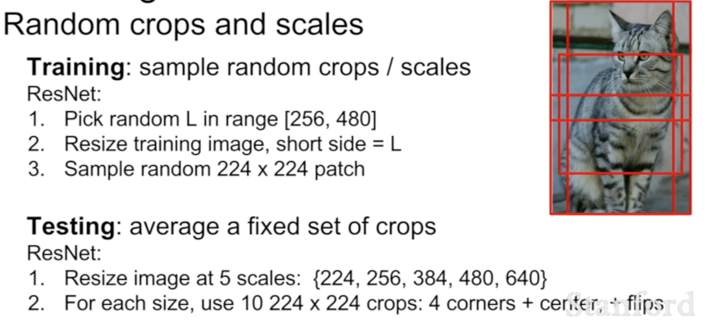
• during testing, average out the stochasticity that was added during training by evaluating with some fixed set of crops (often four corners and the middle and their flips)

Color jittering

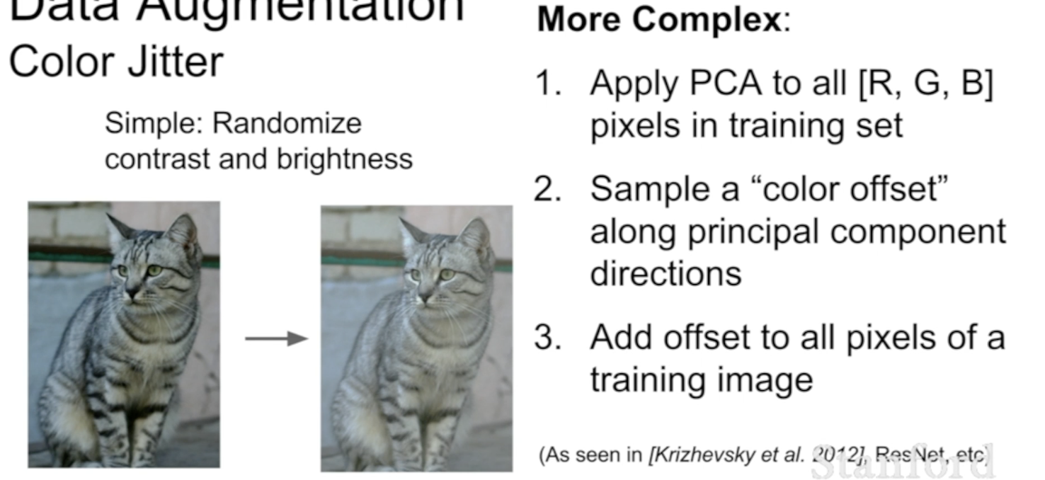
• randomly vary the contrast or brightness during training

---

• data augmentation is a general thing that you can apply to any problem
• think about the way that you can transform the data without changing label

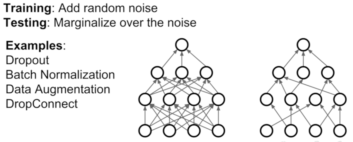
• drop connect: rather than zeroing out the activations, randomly zero out some of the values of weight matrix

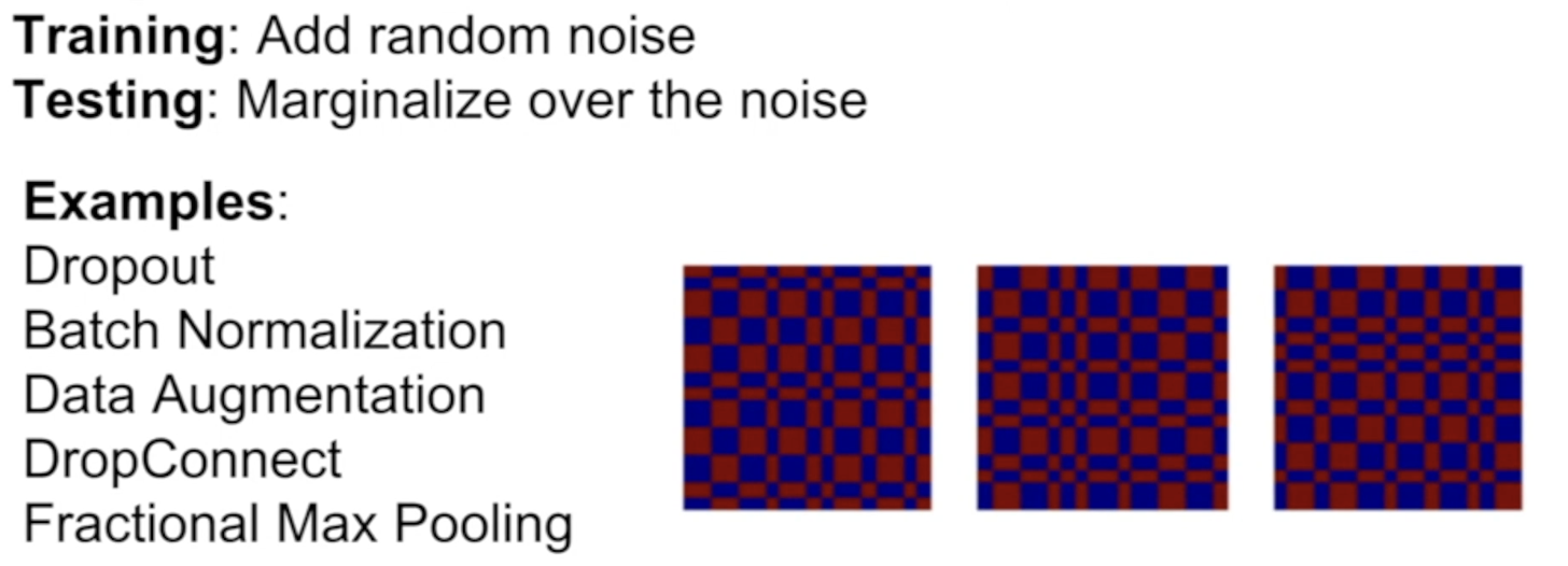
• fractional max pooling: every time we have pooling layer, randomize the regions over which we pool.
  • during test time, average out stochasticity by sticking to some fixed set of pooling regions or drawing many samples and averaging over them
  • not commonly used

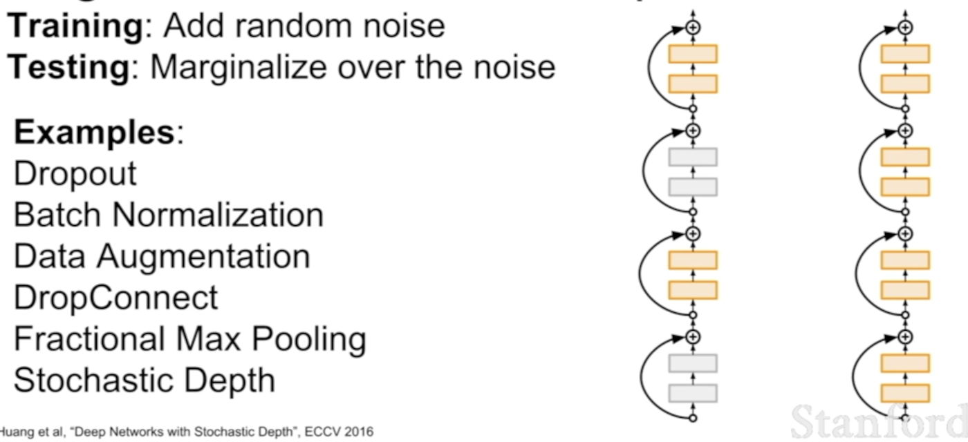
• stochastic depth: a very deep network, and randomly drop layers from the network during training and only use subset of layers during training
  • during test time, use the whole network
  • similar effect as dropout

Transfer Learning

• with regularization, we can reduce the gap between train and test error
• and sometimes you overfit b/c you don't have enough data
  • regularization and transfer learning are the ways to combat this
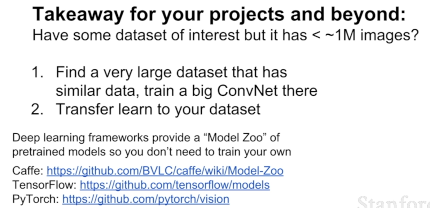
• busts the myth that you need a lot of data to train a CNN
  

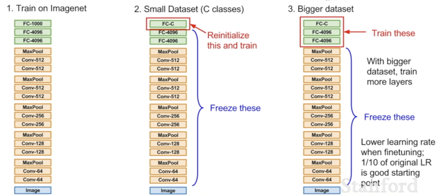
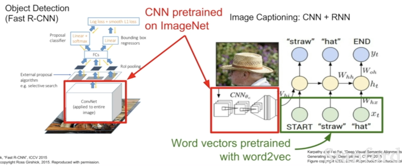
1. Take CNN and train it on a large dataset (ex. ImageNet)
2. Apply features from this dataset to some small dataset you care about
   • ex) instead of classifying 1000 categories, just classify 10 dog breeds
3. Now reinitialize the last layer(FC-C layer) randomly and freeze the weights of all the previous layers
   • ex) 4096xC matrix
4. train a linear classifier and only train the parameters of this last layer
5. If you have more data, you can fine tune the whole network
   • after learning the last layer for the data, you can try to update the whole network

• when updating the network, you want to drop the learning rate from its initial learning rate
  • b/c the original parameters in this network that converged on ImageNet probably worked well generally, and just want to change them a very small amount to tune performance for data set

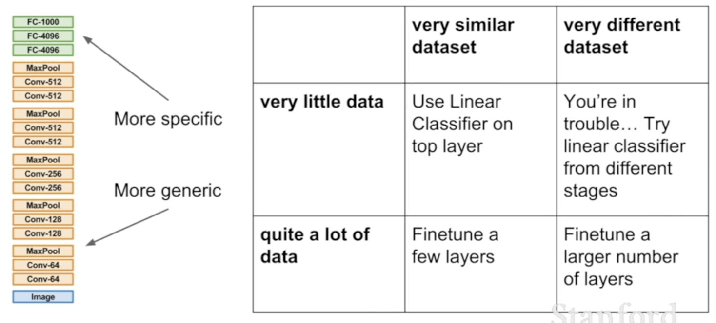
• transfer learning is pervasive(만연한)
  • is a norm rather than exception