네이버 쇼핑 감정분류

데이터 및 라이브러리 로드

import re
import pandas as pd
import numpy as np
import matplotlib.pyplot as plt
import urllib.request
from collections import Counter
from konlpy.tag import Mecab
from sklearn.model_selection import train_test_split
from tensorflow.keras.preprocessing.text import Tokenizer
from tensorflow.keras.preprocessing.sequence import pad_sequences

urllib.request.urlretrieve("https://raw.githubusercontent.com/bab2min/corpus/master/sentiment/naver_shopping.txt", filename="ratings_total.txt")

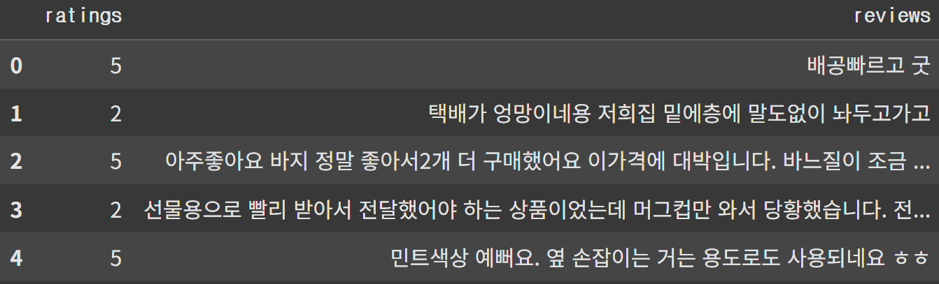
total_data=pd.read_table('ratings_total.txt',names=['ratings','reviews'])
len(total_data)

총 200,000개 데이터

데이터의 구조

데이터 전처리

중복된 데이터 제거

total_data.drop_duplicates(subset=['reviews'], inplace=True)
len(total_data)

중복된 데이터 제거 후 데이터 개수 199,908개

훈련, 테스트 데이터 분리

train_data, test_data=train_test_split(total_data, test_size=0.25, random_state=42)

레이블 분포 확인

train_data['label'].value_counts().plot(kind='bar')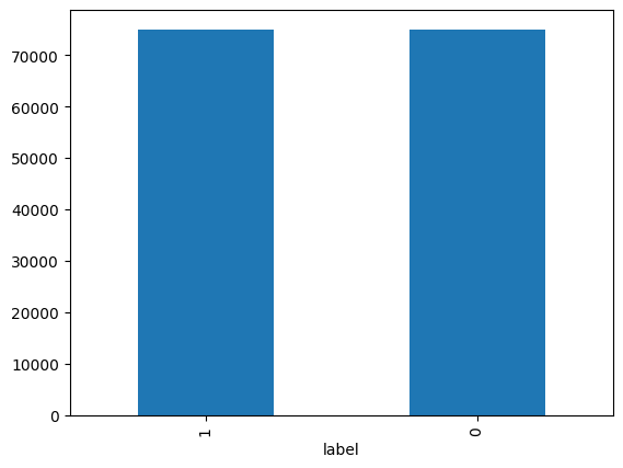

train_data.groupby('label').size().reset_index(name='count')

	label	count
0	0	74918
1	1	75013

텍스트 전처리

정규표현식을 이용한 텍스트 전처리

train_data['reviews']=train_data['reviews'].str.replace('[^ㄱ-ㅎㅏ-ㅣ가-힣] ','', regex=True)
train_data['reviews'].replace('', np.nan, inplace=True)

테스트 데이터에도 앞 과정과 같은 방법 수행

test_data.drop_duplicates(subset = ['reviews'], inplace=True) # 중복 제거
test_data['reviews'] = test_data['reviews'].str.replace("[^ㄱ-ㅎㅏ-ㅣ가-힣 ]","", regex=True) # 정규 표현식 수행
test_data['reviews'].replace('', np.nan, inplace=True) # 공백은 Null 값으로 변경
test_data = test_data.dropna(how='any') # Null 값 제거
print('전처리 후 테스트용 샘플의 개수 :',len(test_data))

전처리 후 테스트용 샘플의 개수 : 49977

형태소 분석, 불용어 처리

mecab=Mecab()

stopwords = ['도', '는', '다', '의', '가', '이', '은', '한', '에', '하', '고', '을', '를', '인', '듯', '과', '와', '네', '들', '듯', '지', '임', '게']

# 훈련 데이터
train_data['tokenized']=train_data['reviews'].apply(mecab.morphs)
train_data['tokenized']=train_data['tokenized'].apply(lambda x:[item for item in x if item not in stopwords])

# 테스트 데이터
test_data['tokenized'] = test_data['reviews'].apply(mecab.morphs)
test_data['tokenized'] = test_data['tokenized'].apply(lambda x: [item for item in x if item not in stopwords])

긍정, 부정리뷰 탐색

부정리뷰에서 많이 쓰인 단어

negative_words=np.hstack(train_data[train_data.label==0]['tokenized'].values)

print(negative_word_count.most_common(20))

[('.', 54967), ('네요', 31738), ('는데', 20229), ('안', 19731), ('어요', 15095), ('있', 13201), ('너무', 12983), ('했', 11885), ('좋', 9801), ('배송', 9673), ('같', 9004), ('어', 8968), ('거', 8867), ('구매', 8867), ('없', 8674), ('아요', 8620), ('습니다', 8429), ('그냥', 8353), ('되', 8346), ('잘', 8020)]

긍정리뷰에서 많이 쓰인 단어

positive_words=np.hstack(train_data[train_data.label==1]['tokenized'].values)

positive_word_count = Counter(positive_words)
print(positive_word_count.most_common(20))

[('좋', 39438), ('아요', 21107), ('네요', 19783), ('.', 19403), ('어요', 19115), ('잘', 18598), ('구매', 16153), ('습니다', 13319), ('있', 12389), ('배송', 12258), ('는데', 11660), ('했', 10158), ('합니다', 9808), ('먹', 9642), ('재', 9258), ('너무', 8388), ('!', 8339), ('같', 7866), ('만족', 7246), ('~', 6940)]

긍정, 부정의 길이 분포 확인

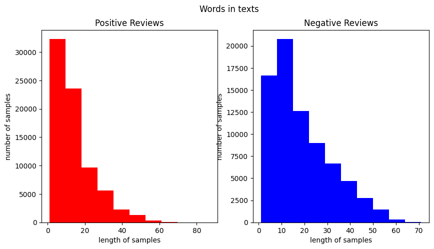
fig,(ax1,ax2) = plt.subplots(1,2,figsize=(10,5))
text_len = train_data[train_data['label']==1]['tokenized'].map(lambda x: len(x))
ax1.hist(text_len, color='red')
ax1.set_title('Positive Reviews')
ax1.set_xlabel('length of samples')
ax1.set_ylabel('number of samples')
print('긍정 리뷰의 평균 길이 :', np.mean(text_len))

text_len = train_data[train_data['label']==0]['tokenized'].map(lambda x: len(x))
ax2.hist(text_len, color='blue')
ax2.set_title('Negative Reviews')
fig.suptitle('Words in texts')
ax2.set_xlabel('length of samples')
ax2.set_ylabel('number of samples')
print('부정 리뷰의 평균 길이 :', np.mean(text_len))
plt.show()

긍정 리뷰의 평균 길이 : 14.391118872728727
부정 리뷰의 평균 길이 : 18.350836915027095

토큰화

토큰화된 데이터로 훈련, 테스트 데이터 분리

X_train = train_data['tokenized'].values
y_train = train_data['label'].values
X_test= test_data['tokenized'].values
y_test = test_data['label'].values

정수 인코딩

tokenizer=Tokenizer()
tokenizer.fit_on_texts(X_train)

희귀 단어 제거

희귀 단어 비율 확인

threshold=2
total_cnt=len(tokenizer.word_index)
rare_cnt=0
total_freq=0
rare_freq=0

for key, value in tokenizer.word_counts.items():
  total_freq+=value
  if value<threshold:
    rare_cnt+=1
    rare_freq+=value

print('단어 집합(vocabulary)의 크기 :',total_cnt)
print('등장 빈도가 %s번 이하인 희귀 단어의 수: %s'%(threshold - 1, rare_cnt))
print("단어 집합에서 희귀 단어의 비율:", (rare_cnt / total_cnt)*100)
print("전체 등장 빈도에서 희귀 단어 등장 빈도 비율:", (rare_freq / total_freq)*100)

단어 집합(vocabulary)의 크기 : 43031
등장 빈도가 1번 이하인 희귀 단어의 수: 20236
단어 집합에서 희귀 단어의 비율: 47.02656224582278
전체 등장 빈도에서 희귀 단어 등장 빈도 비율: 0.8245023385210378

vocab_size=total_cnt-rare_cnt+2
vocab_size

22797

정수 인코딩

22,797 보다 큰 숫자들은 OOV로 변환

tokenizer=Tokenizer(vocab_size, oov_token='OOV')
tokenizer.fit_on_texts(X_train)
X_train=tokenizer.texts_to_sequences(X_train)
X_test=tokenizer.texts_to_sequences(X_test)

print(X_train[:3])

[[71, 147, 2062, 315, 14826, 276, 77, 7, 251, 180, 146, 834, 3038, 658, 3, 83, 67, 218, 42, 1398, 167, 4, 7], [509, 2760, 2, 8838, 2734, 2, 2511, 352, 3039, 266, 2438, 39, 493, 3], [48, 25, 868, 102, 36, 2421, 172, 8, 11, 8366, 5, 1369, 31, 149, 336, 45, 63, 172, 149, 8, 1977, 3, 2, 2, 118, 174, 1437, 302, 2, 2, 128, 144, 2, 6476]]

데이터 길이 분포 확인

print(max((len(review) for review in X_train)))
print(sum(map(len, X_train))/len(X_train))
plt.hist([len(review) for review in X_train], bins=50)
plt.xlabel('length of samples')
plt.ylabel('number of samples')
plt.show()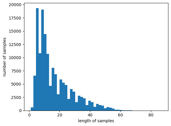

패딩

def below_threshold_len(max_len, nested_list):
  count=0
  for sentence in nested_list:
    if len(sentence)<=max_len:
      count+=1
  print('전체 샘플 중 길이가 %s 이하인 샘플의 비율: %s'%(max_len, (count / len(nested_list))*100))

max_len=80
below_threshold_len(max_len, X_train)

전체 샘플 중 길이가 80 이하인 샘플의 비율: 99.99866605305107

X_train=pad_sequences(X_train, maxlen=max_len)
X_test=pad_sequences(X_test, maxlen=max_len)

GRU 모델

모델 설계

from tensorflow.keras.layers import Embedding, Dense, GRU
from tensorflow.keras.models import Sequential
from tensorflow.keras.models import load_model
from tensorflow.keras.callbacks import EarlyStopping, ModelCheckpoint

embedding_dim=100
hidden_units=128

model=Sequential()
model.add(Embedding(vocab_size, embedding_dim))
model.add(GRU(hidden_units))
model.add(Dense(1, activation='sigmoid'))

es=EarlyStopping(monitor='val_loss', mode='min', verbose=1, patience=4)
mc=ModelCheckpoint('best_model.keras', monitor='val_acc', mode='max', verbose=1, save_best_only=True)
model.compile(optimizer='rmsprop', loss='binary_crossentropy', metrics=['acc'])

history=model.fit(X_train, y_train, batch_size=64, epochs=15, validation_split=0.2, callbacks=[es, mc])

테스트 데이터 정확도

loaded_model=load_model('best_model.keras')
print(model.evaluate(X_test, y_test))

0.9139603972434998

모듈화

def sentiment_predict(new_sentence):
  new_sentence = re.sub(r'[^ㄱ-ㅎㅏ-ㅣ가-힣 ]','', new_sentence)
  new_sentence = mecab.morphs(new_sentence)
  new_sentence = [word for word in new_sentence if not word in stopwords]
  encoded = tokenizer.texts_to_sequences([new_sentence])
  pad_new = pad_sequences(encoded, maxlen = max_len)

  score = float(loaded_model.predict(pad_new))
  if(score > 0.5):
    print("{:.2f}% 확률로 긍정 리뷰입니다.".format(score * 100))
  else:
    print("{:.2f}% 확률로 부정 리뷰입니다.".format((1 - score) * 100))

새로운 리뷰 예측

sentiment_predict('이 상품 진짜 좋아요... 저는 강추합니다. 대박')

97.58% 확률로 긍정 리뷰입니다.

sentiment_predict('진짜 배송도 늦고 개짜증나네요. 뭐 이런 걸 상품이라고 만듬?')

99.70% 확률로 부정 리뷰입니다.

sentiment_predict('ㅁㄴㅇㄻㄴㅇㄻㄴㅇ리뷰쓰기도 귀찮아')

88.34% 확률로 부정 리뷰입니다.