
개요
본 블로그 포스팅은 수도권 ICT 이노베이션 스퀘어에서 진행하는 AI 핵심 기술 집중 클래스의 자연어처리(NLP) 강좌 내용을 필자가 다시 복기한 내용에 관한 것입니다.
1. 실습 개요
이전 포스트 NLP-LSTM, GRU (3) : 개체명 인식(NER : Named Entity Recognition)
NLP-LSTM, GRU (3-1) : NER에 CRF(Conditional Random Field) 추가
위 두개 포스트에서 너무 예의없게
학습/검증까지만 수록하고
실제 임의의 데이터를 입력 받았을 때
이게 진짜 잘 NER 태깅이 완료되었는지를 확인하는
추론과정을 포함을 안 시켰었는데
이 과정을 포함시키는 것과
NER 학습/검증용 model_train, model_evaluate 함수도 범용성 있게 재 작성해서 이를 모두 배포하려 한다.
우선 수행 과정은 아래와 같다.
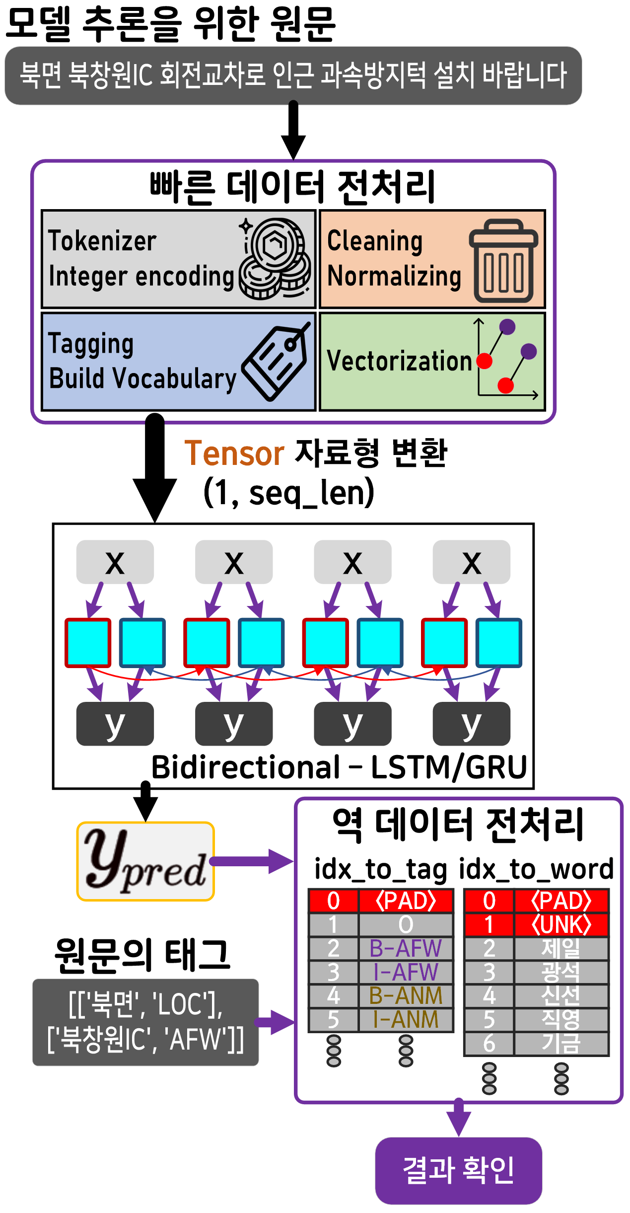
모델 추론 과정에서 사용되는 전처리 함수들은
전처리 과정에서 생성되는 word_to_idx, tag_to_idx의
거울 쌍 딕셔너리인 idx_to_word, idx_to_tag가 꼭 필요하다
그러니 학습/검증이 완료된 이후 평가까지 함께 수행하거나
아니면 위 딕셔너리는 따로 저장하는 것을 권장한다
2. 일반 bi-LSTM/GRU 추론
NLP-LSTM, GRU (3) : 개체명 인식(NER : Named Entity Recognition)
포스트 결과물에 대한 추론 성능을 테스트해보자
먼저 학습이 완료된 이후 모델 저장은 필수다
# 학습된 모델 저장
path = {} #모델별 경로명 저장
for mk in model_key:
    path[mk] = f'{mk}_NER.pth'
    torch.save(models[mk].state_dict(), path[mk])
모델 저장을 완료했으면
# 저장된 모델 불러오기
load_model = {
    'LSTM': Lstm_tagger,  # LSTM 모델 인스턴스 생성
    'GRU': Gru_tagger      # GRU 모델 인스턴스 생성
}
for mk in model_key:
    load_model[mk].load_state_dict(torch.load(path[mk], weights_only=True))
    #추론기는 CPU에서 돌리자
    load_model[mk] = load_model[mk].to('cpu')
모델을 불러오며, 이때 추론은 CPU에서 연산을 수행하고자 한다.
import random
total_docs = len(raw_data)
sample_idx = random.randint(0, total_docs-1)
# 데이터프레임의 항목을 분리 후 리스트 타입으로 변경
sample_doc = raw_data['컨텐츠'].iloc[sample_idx]
# 개체 : 개체 라벨링 의 태그 정보는 따로 추출한다.
sample_tag = raw_data['개체'].iloc[sample_idx]
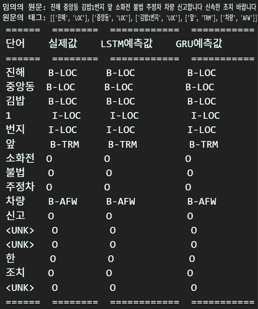
print(f'임의의 원문: {sample_doc}')
print(f'원문의 태그: {sample_tag}')임의의 원문은 비교를 용이하기 위해
태그 정보도 함께 있는 파일로부터 추출해왔다
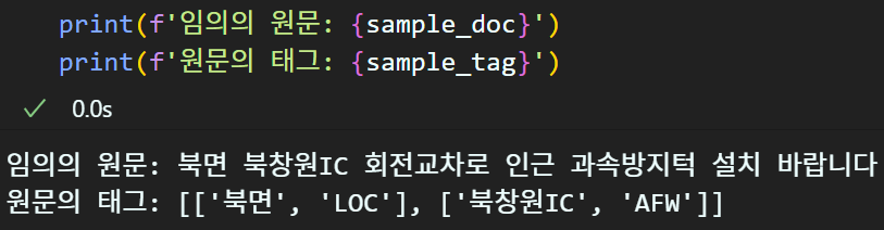
대략 원문/태그는 위 사진과 같으며
sample_idx를 랜덤값으로 계속 돌릴 수 있으니
여러번 테스트가 가능하게 하자
빠른 전처리
원문 딱 1개밖에 없으니 빠르게 전처리를 수행하자
def convert_model_input(x_data, word_tokenizer, word_to_idx, context_length):
    token_x_data = tokenize([x_data], word_tokenizer)
    e_token = text_to_sequences(token_x_data, word_to_idx)
    pad_token = pad_seq_x(e_token, context_length)
    t_pad_token = torch.tensor(pad_token, dtype=torch.long)

    return t_pad_token # 출력물은 (1, seq_len)의 텐서 자료형

def convert_tag_label(x_data, tags, word_tokenizer, tag_to_idx, context_length):
    temp = tokenize([x_data], word_tokenizer)
    token_label, _ = BIO_tagging(temp, [tags], word_tokenizer)
    e_label = text_to_sequences(token_label, tag_to_idx, spec_token='O')
    pad_label = pad_seq_x(e_label, context_length)
    t_pad_label = torch.tensor(pad_label, dtype=torch.long)

    return t_pad_label # 출력물은 (1, seq_len)의 텐서 자료형
전처리 함수 모음 NLP_pp.py의 각종 함수들을 불러와서 빠르게
원문, 태그에 대한 전처리를 수행하자
태그를 원문과 함께 전처리를 수행하면 BIO태깅 규칙을 준수한 라벨링 데이터를 얻을 수 있다.
설계함 함수는 아래의 코드로 사용할 수 있다.
t_doc = convert_model_input(sample_doc, word_tokenizer, word_to_idx, context_length)
print()
t_label = convert_tag_label(sample_doc, sample_tag, word_tokenizer, tag_to_idx, context_length)
모델 추론하기
# 모델별 추론 수행행
outputs = {}
for mk in model_key:
    load_model[mk].eval()

    with torch.no_grad():
        # 모델의 출력값 연산
        output = load_model[mk](t_doc)
        # 모델의 출력값은 (bs, seq_len, tag_dim)이니 argmax로 best_pred연산
        best_pred = output.argmax(dim=2)
        outputs[mk] = best_pred[0].cpu().numpy() #numpy자료형변환
다음으로 Bi-LSTM, Bi-GRU 두개의 모델이 있으니
각각 추론을 진행하자
추론 결과는 numpy 자료형으로 변환하여 딕셔너리에 각각 저장한다
추론 결과 분석
# 출력할 데이터를 저장할 리스트 생성
table_data = []
x_data = t_doc[0].cpu().numpy()
y_label = t_label[0].cpu().numpy()
for word, tag, lstm_pred, gru_pred in zip(x_data, y_label,
outputs['LSTM'],
outputs['GRU']):
if word != 0: #PAD 토큰 제외
table_data.append([idx_to_word[word], idx_to_tag[tag],
idx_to_tag[lstm_pred], idx_to_tag[gru_pred]])
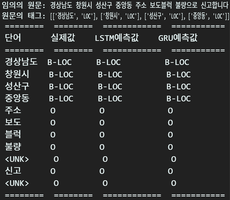
# 테이블 헤더
headers = ["단어", "실제값", "LSTM예측값", "GRU예측값"]
# tabulate를 사용하여 출력
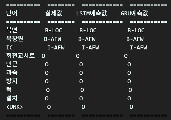
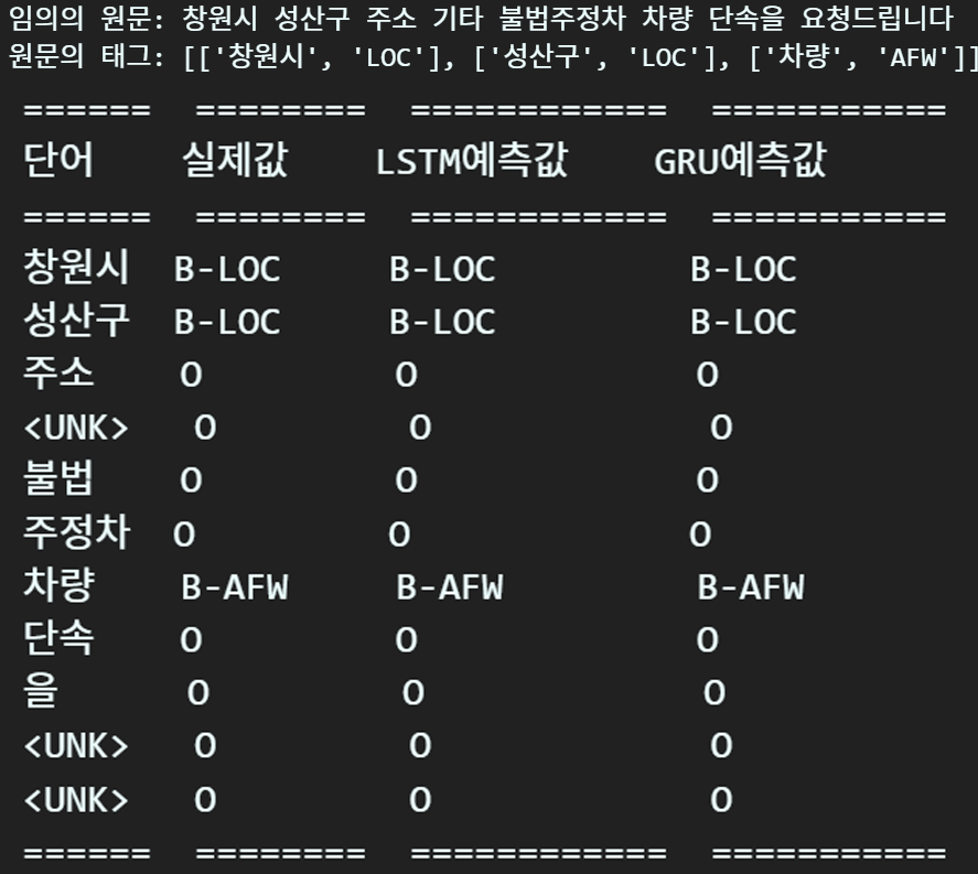
print(tabulate(table_data, headers=headers, tablefmt="rst"))추론 결과는 보기 좋게 tabulate라이브러리를 사용하여
원문, 정답지, 각 모델별 추론결과
를 비교분석하자

3. CRF+bi-LSTM/GRU 추론
NLP-LSTM, GRU (3-1) : NER에 CRF(Conditional Random Field) 추가
이 포스트에서도 수행했던
CRF+Bi-LSTM/GRU 버전도 동일하게 모델 저장/로드를 수행하자
# 학습된 모델 저장
path = {} #모델별 경로명 저장
for mk in model_key:
    path[mk] = f'{mk}_NER.pth'
    torch.save(models[mk].state_dict(), path[mk])
# 저장된 모델 불러오기
load_model = {
'BiLSTM+CRF': Lstm_tagger, # LSTM 모델 인스턴스 생성
'BiGRU+CRF': Gru_tagger # GRU 모델 인스턴스 생성
}
for mk in model_key:
load_model[mk].load_state_dict(torch.load(path[mk], weights_only=True))
#추론기는 CPU에서 돌리자
load_model[mk] = load_model[mk].to('cpu')그 다음 임의의 원문을 불러오는 과정은 동일하다
import random
total_docs = len(raw_data)
sample_idx = random.randint(0, total_docs-1)

# 데이터프레임의 항목을 분리 후 리스트 타입으로 변경
sample_doc = raw_data['컨텐츠'].iloc[sample_idx]
# 개체 : 개체 라벨링 의 태그 정보는 따로 추출한다.
sample_tag = raw_data['개체'].iloc[sample_idx]

print(f'임의의 원문: {sample_doc}')
print(f'원문의 태그: {sample_tag}')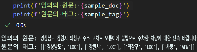
빠른 전처리
전처리 함수는 챕터 2에 기재한 함수와 동일하다
t_doc = convert_model_input(sample_doc, word_tokenizer, word_to_idx, context_length)
print()
t_label = convert_tag_label(sample_doc, sample_tag, word_tokenizer, tag_to_idx, context_length)
모델 추론
# 모델별 추론 수행행
outputs = {}
for mk in model_key:
    load_model[mk].eval()

    with torch.no_grad():
        # 모델의 출력값 연산
        output = load_model[mk](t_doc)
        # 모델의 출력값은 2중 리스트 형태 -> numpy로 변환
        outputs[mk] = np.array(output[0])
CRF+Bi-LSTM/GRU의 평가모드 추론결과는 2중 리스트이니 이를 살짝 주의하자
추론 결과 분석
코드는 챕터 2와 같으나 한번 더 붙여넣겠다.
# 출력할 데이터를 저장할 리스트 생성
table_data = []

x_data = t_doc[0].cpu().numpy()
y_label = t_label[0].cpu().numpy()

print(x_data.shape)

for word, tag, lstm_pred, gru_pred in zip(x_data, y_label,
                                          outputs['BiLSTM+CRF'],
                                          outputs['BiGRU+CRF']):
    if word != 0: #PAD 토큰 제외
        table_data.append([idx_to_word[word], idx_to_tag[tag],
                           idx_to_tag[lstm_pred], idx_to_tag[gru_pred]])

# 테이블 헤더
headers = ["단어", "실제값", "LSTM예측값", "GRU예측값"]

# tabulate를 사용하여 출력
print(tabulate(table_data, headers=headers, tablefmt="rst"))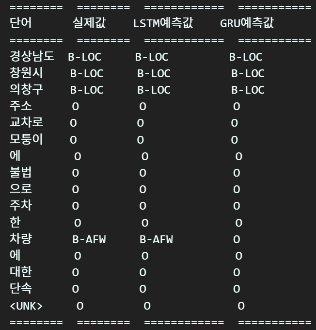

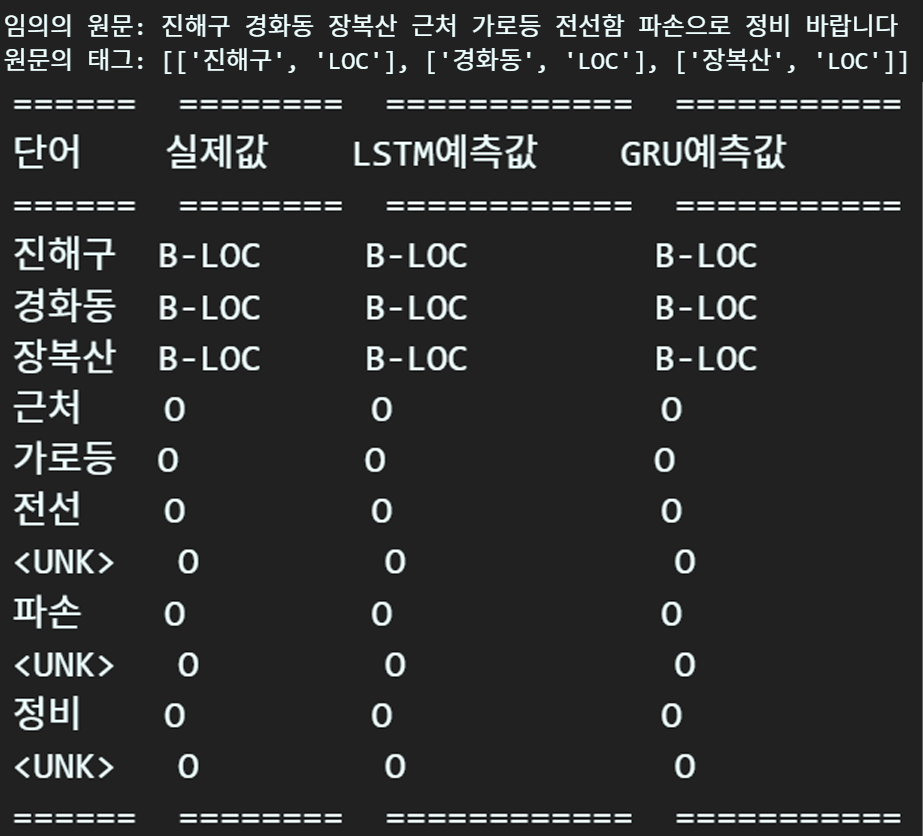
이정도면 결과물은 모두 훌륭한 듯 싶다
3. 마무리
NER 실습을 위해 사용한 두개의 ipynb파일과
모델 훈련/실습 함수는 모두
https://github.com/tbvjvsladla/NER_tagging/tree/main
여기에 업로드 하였다.
특히 Ner_trainer.py파일은
모델 훈련/검증에 사용하는 model_train, model_evaluate 함수가
Bi-LSTM/GRU, CRF+Bi-LSTM/GRU에 대응할 수 있도록
범용적으로 설계를 진행했다.
이로써 NER 추론까지 모두 마치도록 하겠다.