복잡한 데이터 표현하기
객체지향 API
그래프는 그리는 방법은 pyplot 방식과 객체지향 API방식 두가지가 존재함
pyplot 방식으로 그래프 그리기
plt.plot([1, 4, 9, 16])
plt.title('simple line graph')
plt.show()
객체지향 API 방식으로 그래프 그리기
fig라는 틀에 ax라는 종이를 놓고 그래프를 그린다고 생각
fig, ax = plt.subplots()
ax.plot([1, 4, 9, 16])
ax.set_title('simple line graph')
fig.show()
하나의 그래프를 간단하게 그릴 때는 pyplot, 그래프를 여러개 그리거나 꾸미려면 객체지향 API 방식을 사용
그래프에 한글 출력하기
- 폰트설치 코랩에서 폰트설치 → 런타임 → 런타임 다시시작을 해야 적용완료됨
import sys
if 'google.colab' in sys.modules:
    !echo 'debconf debconf/frontend select Noninteractive' | debconf-set-selections
    # 나눔 폰트를 설치합니다.
    !sudo apt-get -qq -y install fonts-nanum
    import matplotlib.font_manager as fm
    fm._rebuild()
폰트 지정하기(1) : font.family 속성
맷플롯립의 기본 폰트는 영문 sans-serif 폰트
# 나눔고딕 폰트로 변경
plt.rcParams['font.family'] = 'NanumGothic'
폰트 지정하기(2) : rc() 함수
# 나눔바른고딕 폰트로 변경 및 폰트 크기변경
plt.rc('font', family='NanumBarunGothic', size=11)
폰트 변경사항 확인
print(plt.rcParams['font.family'], plt.rcParams['font.size'])시스템 기본 폰트 확인
from matplotlib.font_managerimport findSystemFonts
findSystemFonts()
도서 개수 산점도 그리기
- 데이터 다운로드 및 확인
import gdown
gdown.download('https://bit.ly/3pK7iuu', 'ns_book7.csv', quiet=False)

import pandas as pd
ns_book7 = pd.read_csv('ns_book7.csv', low_memory=False)
ns_book7.head()
출판사 목록 만들기
# 상위 30개의 출판사 목록생성
top30_pubs = ns_book7['출판사'].value_counts()[:30]
top30_pubs

# 상위 30개에 해당하는 출판사면 True 그렇지 않으면 False 반환
top30_pubs_idx = ns_book7['출판사'].isin(top30_pubs.index)

# 상위 30개 출판사의 발행 도서 개수 출력
top30_pubs_idx.sum()
무작위 데이터 고르기
ns_book8 = ns_book7[top30_pubs_idx].sample(1000, random_state=42)
ns_book8.head()
산점도 그리기
fig, ax = plt.subplots(figsize=(10, 8))
ax.scatter(ns_book8['발행년도'], ns_book8['출판사'])
ax.set_title('출판사별 발행도서')
fig.show()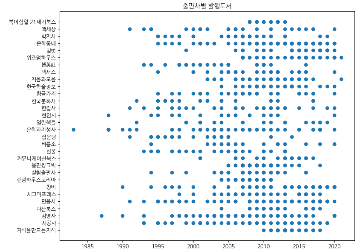
값에 따라 마커 크기 다르게 나타내기
rcParams[’linex.markersize’]를 이용하며 기본값은 6
fig, ax = plt.subplots(figsize=(10, 8))
# 대출건수가 많은 도서를 상대적으로 크게 나타냄
ax.scatter(ns_book8['발행년도'], ns_book8['출판사'], s=ns_book8['대출건수'])
ax.set_title('출판사별 발행 도서')
fig.show()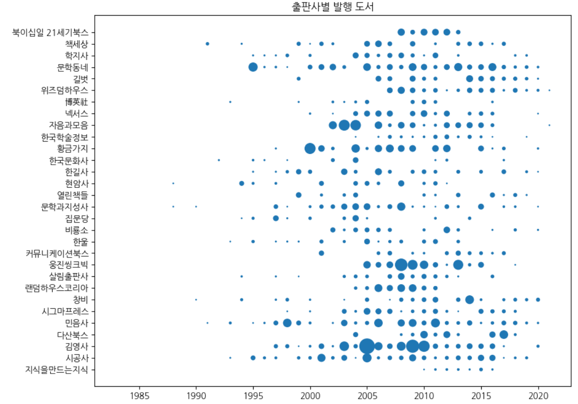
마커꾸미기
- 투명도 조절하기 : alpha 매개변수
- 마커 테두리 색 바꾸기: edgecolor 기본값은 ‘face’
- 마커 테두리 선 두께 바꾸기 : linewidths 마커 테두리 선의 두께를 결정 기본값은 1.5
- 산점도 색 바꾸기 : c 산점도의 색을 지정, 데이터의 개수와 동일한 길이의 배열을 전달하면 각 데이터를 다른 색깔로 그릴 수 있음
fig, ax = plt.subplots(figsize=(10, 8))
ax.scatter(ns_book8['발행년도'], ns_book8['출판사'],
           linewidths=0.5, edgecolors='k', alpha=0.3,
           s=ns_book8['대출건수']*2, c=ns_book8['대출건수'])
ax.set_title('출판사별 발행도서')
fig.show()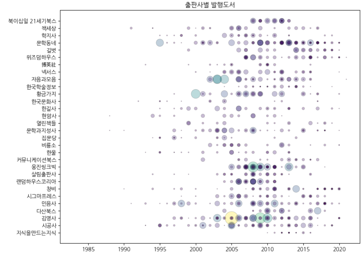
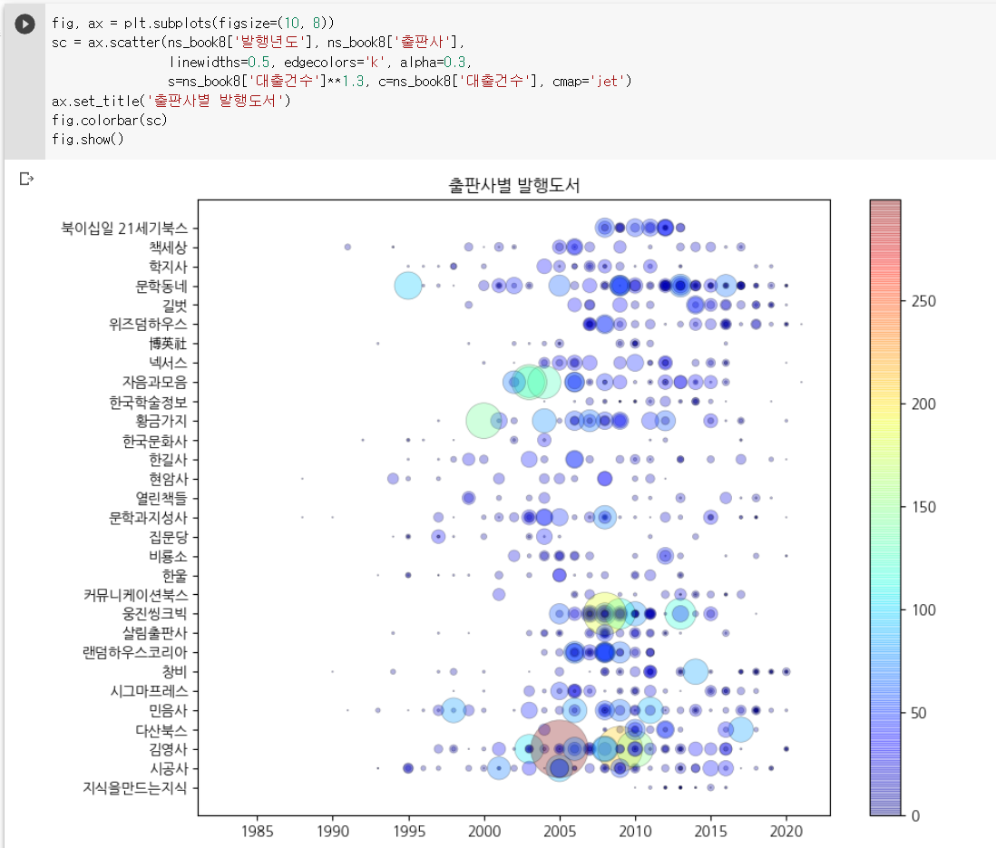
값에 따라 색상 표현하기 : 컬러맵
scatter()함수는 기본값인 viridis 컬러맵으로 표현, 자주 사용하는 컬러맵은 jet 낮은 값일수록 짙은 파란색 높은 값일수록 노란색 → 빨간색으로 바뀜
fig, ax = plt.subplots(figsize=(10, 8))
sc = ax.scatter(ns_book8['발행년도'], ns_book8['출판사'],
                linewidths=0.5, edgecolors='k', alpha=0.3,
                s=ns_book8['대출건수']**1.3, c=ns_book8['대출건수'], cmap='jet')
ax.set_title('출판사별 발행도서')
fig.colorbar(sc)
fig.show()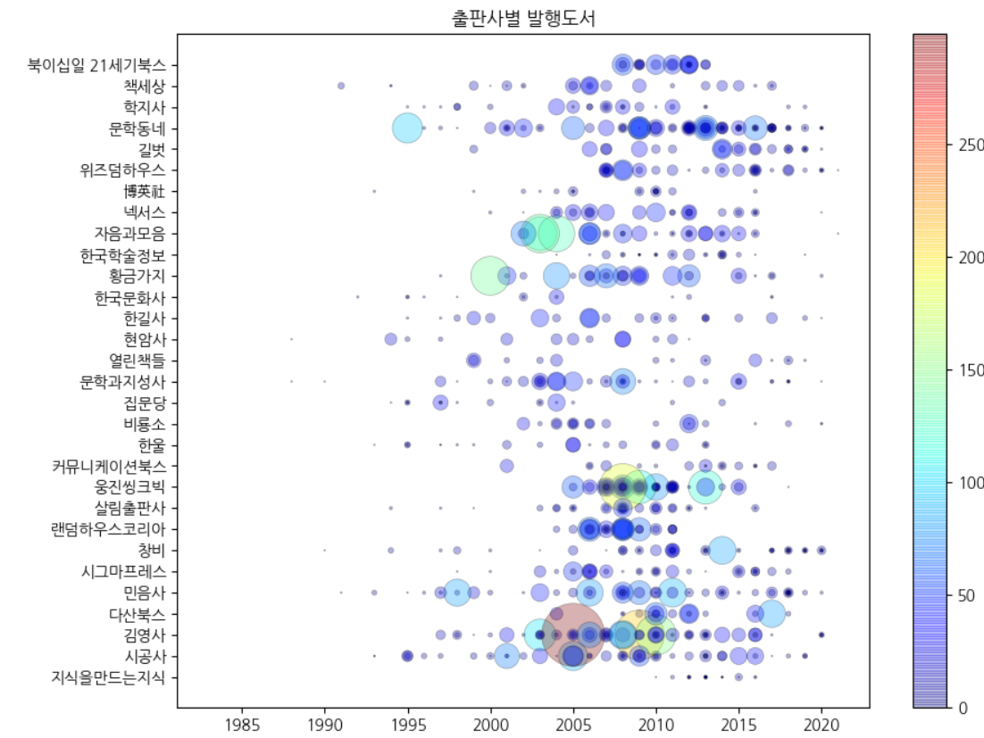
함수
| 함수 | 기능 |
|---|---|
| matplotlib.pyplot.rc() | rcParams 객체의 값을 설정 |
| Figure.colorbar() | 그래프에 컬러 막대 추가 |
맷플롯립의 고급 기능 배우기
데이터 불러오기
import gdown
gdown.download('https://bit.ly/3pK7iuu', 'ns_book7.csv', quiet=False)

import pandas as pd
ns_book7 = pd.read_csv('ns_book7.csv', low_memory=False)
ns_book7.head()
하나의 피겨에 여러 개의 선 그래프 그리기
- 그래프에 필요한 데이터 추출
# 출판사에 대한 발행년도 별 대출건수 그래프 그리기
# 상위 30위 정도 출판사 추출
top30_pubs = ns_book7['출판사'].value_counts()[:30]
top30_pubs_idx = ns_book7['출판사'].isin(top30_pubs.index)

# 상위 30위에 해당하는 출판사, 발행년도, 대출건수 열만 추출
ns_book9 = ns_book7[top30_pubs_idx][['출판사', '발행년도','대출건수']]

# 출판사와 발행년도 열을 기준으로 행을 모은 후 대출건수 열의 합
ns_book9 = ns_book9.groupby(by=['출판사', '발행년도']).sum()

# 인덱스 초기화
ns_book9 = ns_book9.reset_index()
ns_book9[ns_book9['출판사'] === '황금가지'].head()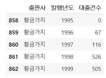
선 그래프 2개 그리기
line1 = ns_book9[ns_book9['출판사'] == '황금가지']
line2 = ns_book9[ns_book9['출판사'] == '비룡소']

fig, ax = plt.subplots(figsize=(8, 6))
ax.plot(line1['발행년도'], line1['대출건수'], label='황금가지')
ax.plot(line2['발행년도'], line2['대출건수'], label='비룡소')
ax.set_title('연도별 대출건수')
# 범례 추가
ax.legend()
fig.show()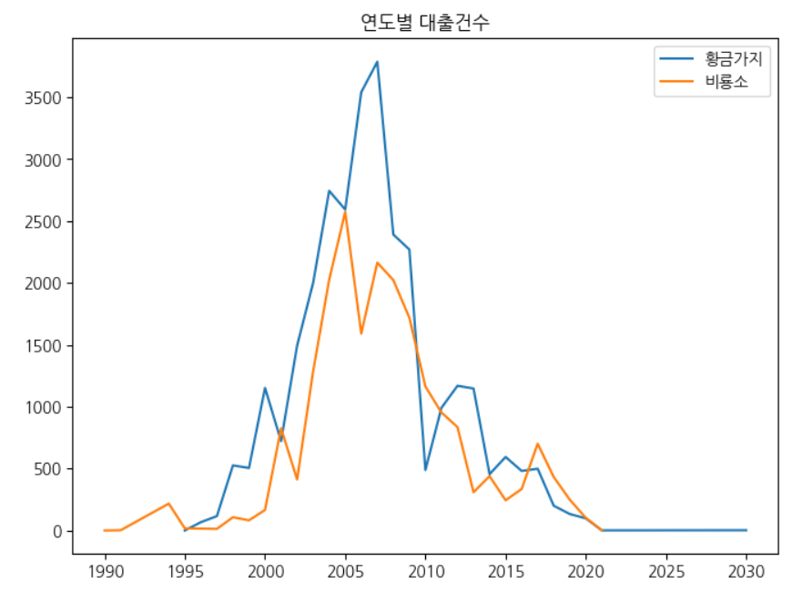
선그래프 5개 그리기
x, y 축의 범위를 지정하는 메서드는 set_xlim, set_ylim을 사용
fig, ax = plt.subplots(figsize=(8, 6))
for pub in top30_pubs.index[:5]:
	line = ns_book9[ns_book9['출판사'] == pub]
	ax.plot(line['발행년도'], line['대출건수'], label=pub)
ax.set_title('연도별 대출건수')
ax.legend()
# x축의 범위 선택
ax.set_xlim(1985, 2025)
fig.show()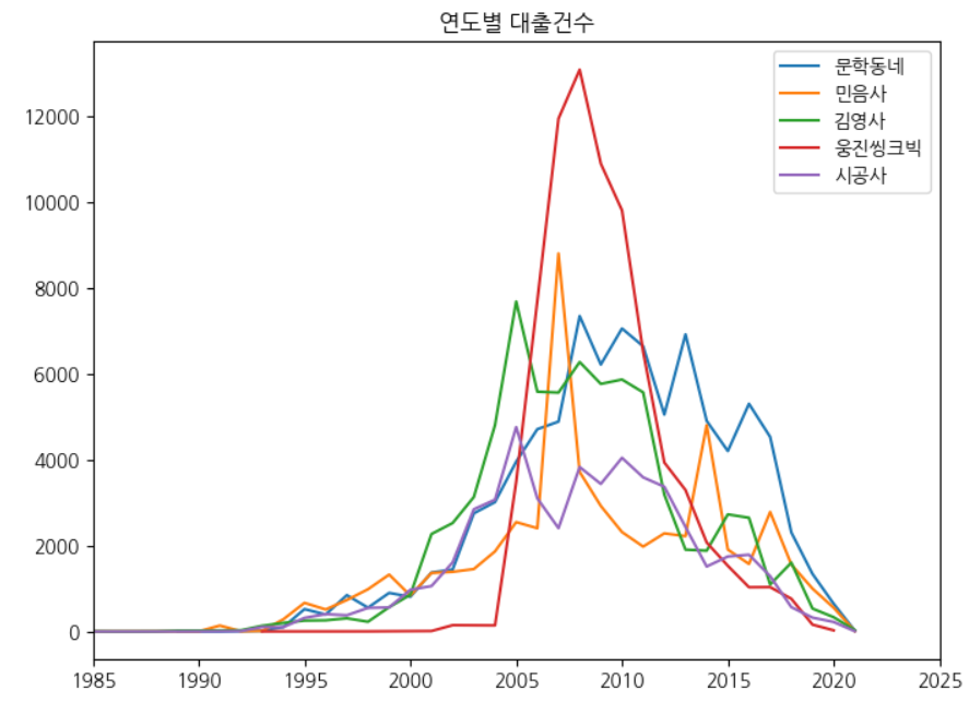
스택 영역 그래프 : stackplot() 함수
하나의 선 그래프 위에 다른 선 그래프를 차례대로 쌓는 것
-
pivot_table() 메서드로 각 ‘발행년도’ 열의 값을 열로 변경
ns_book10 = ns_book9.pivot_table(index='출판사', columns='발행년도')
ns_book10.head()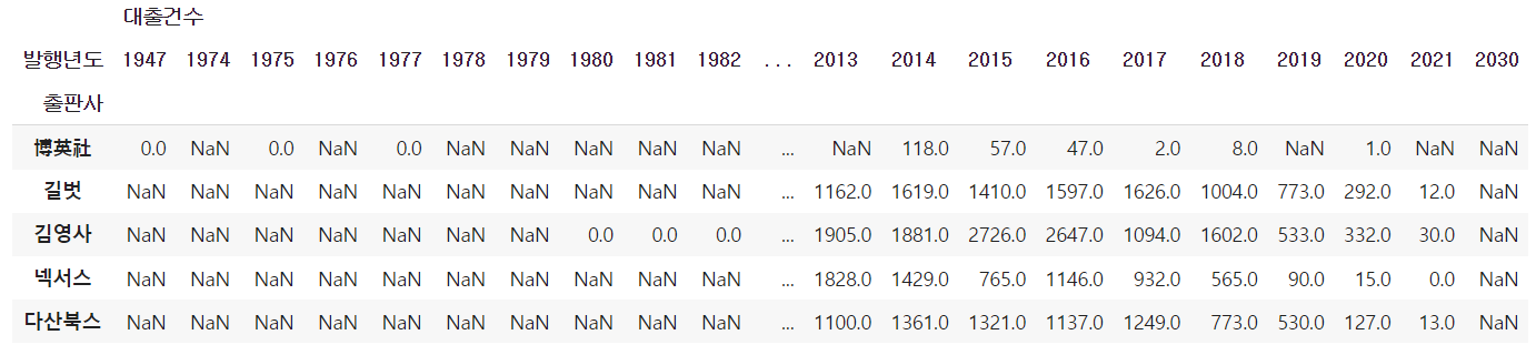
-
‘발행년도’ 열을 리스트 형태로 변경
top10_pubs = top30_pubs.index[:10] # 연도로 구성된 두 번째 항목만 가져옴 year_cols = ns_book10.columns.get_level_values(1) -
stackplot() 메서드로 스택 영역 그래프 그리기
fig, ax = plt.subplots(figsize=(8, 6))
ax.stackplot(year_cols, ns_book10.loc[top10_pubs].fillna(0), labels=top10_pubs)
ax.set_title('연도별 대출건수')
# 범례 왼쪽 상단
ax.legend(loc='upper left')
ax.set_xlim(1985, 2025)
fig.show()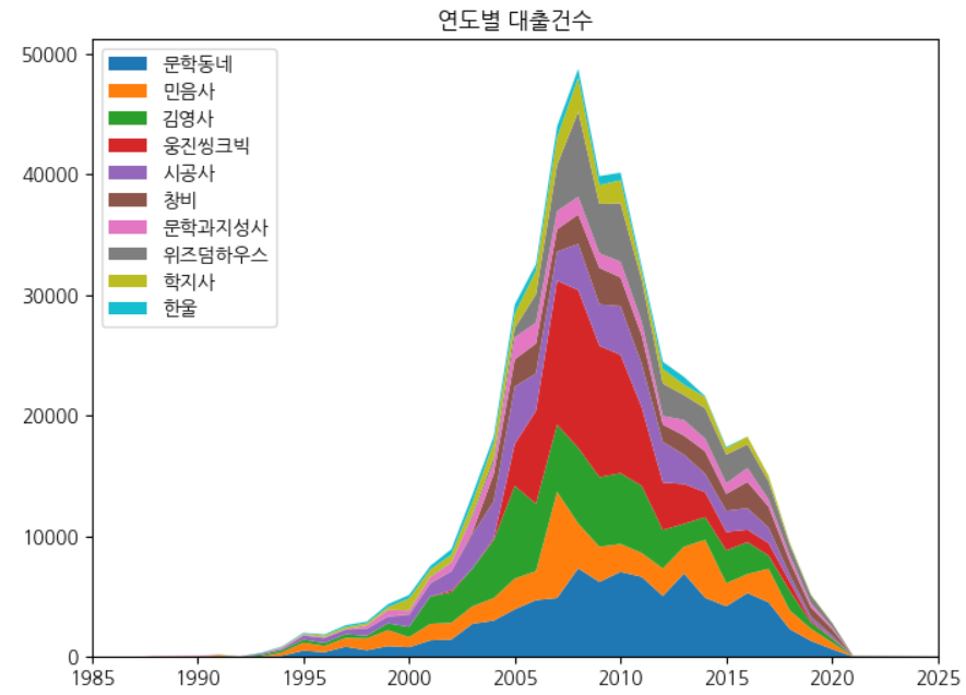
하나의 피겨에 여러 개의 막대 그래프 그리기
fig, ax = plt.subplots(figsize=(8, 6))
ax.bar(line1['발행년도'], line1['대출건수'], label='황금가지')
ax.bar(line2['발행년도'], line2['대출건수'], label='비룡소')
ax.set_title('년도별 대출건수')
ax.legend()
fig.show()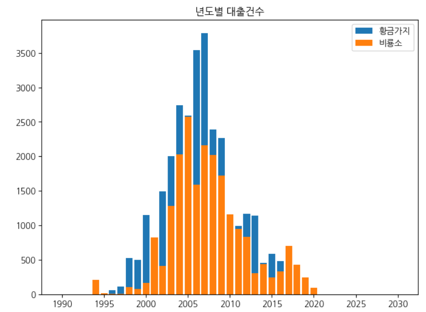
두 막대를 나란히 그리기
fig, ax = plt.subplots(figsize=(8, 6))
ax.bar(line1['발행년도']-0.2, line1['대출건수'], width=0.4, label='황금가지')
ax.bar(line2['발행년도']+0.2, line2['대출건수'], width=0.4, label='비룡소')
ax.set_title('년도별 대출건수')
ax.legend()
fig.show()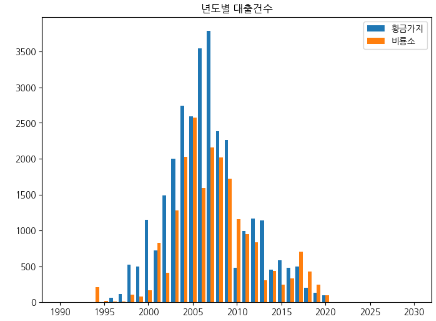
스택 막대 그래프 그리기
stackplot과 달리 막대 그래프는 쌓는 방법은 없지만 수동으로 막대를 쌓음
height1 = [5, 4, 7, 9, 8]
height2 = [3, 2, 4, 1, 2]
plt.bar(range(5), height1, width=0.5)
plt.bar(range(5), height2, bottom=height1, width=0.5)
plt.show()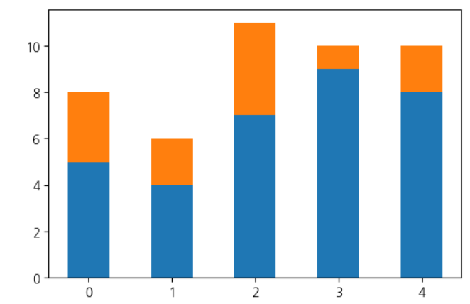
그래프를 그릴때마다 막대의 시작 위치를 계속 누적하여 보관해야 하기 때문에 번거로움 따라서 그리기 전에 막대의 길이를 누적하고 그래프를 그리기
# zip함수로 양쪽의 데이터를 하나씩 엮어줌 [8, 6, 11, 10, 10]
height3 = [a + b for a, b in zip(height1, height2)]

plt.bar(range(5), height3, width=0.5)
plt.bar(range(5), height1, width=0.5)
plt.show()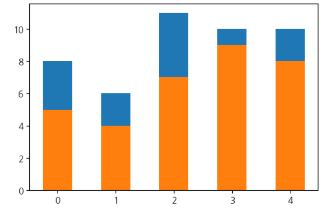
데이터값 누적하여 그리기
판다스의 cumsum() 메서드를 사용하여 값을 누적
ns_book12 = ns_book10.loc[top10_pubs].cumsum()막대 그래프를 쌓을때는 큰 막대를 먼저 그려야함 큰막대가 이전 막대를 덮어쓰기때문
fig, ax = plt.subplots(figsize=(8, 6))
# 누적 합계가 가장 큰 마지막 출판사부터 그림
for i in reversed(range(len(ns_book12))):
    bar = ns_book12.iloc[i]     # 행 추출
    label = ns_book12.index[i]  # 출판사 이름 추출
    ax.bar(year_cols, bar, label=label)
ax.set_title('년도별 대출건수')
ax.legend(loc='upper left')
ax.set_xlim(1985, 2025)
fig.show()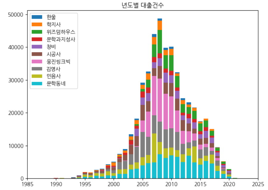
원 그래프 그리기(파이 차트)
data = top30_pubs[:10]
labels = top30_pubs.index[:10]
fig, ax = plt.subplots(figsize=(8, 6))
ax.pie(data, labels=labels)
ax.set_title('출판사 도서 비율')
fig.show()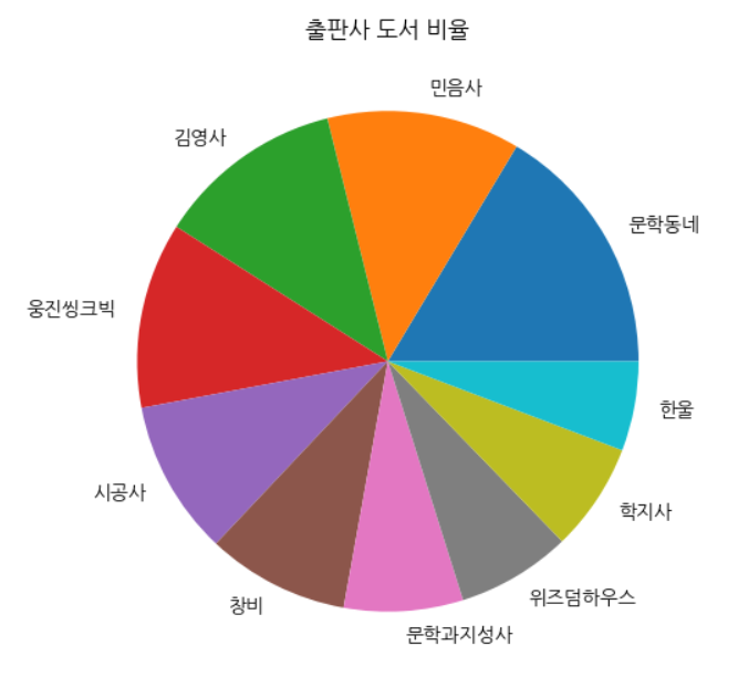
비율 표시 및 부채꼴 강조
fig, ax = plt.subplots(figsize=(8, 6))
ax.pie(data, labels=labels, startangle=90, autopct='%.1f%%', explode=[0.1]+[0]*9)
ax.set_title('출판사 도서 비율')
fig.show()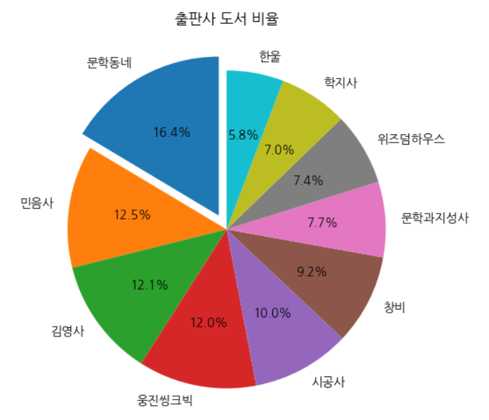
여러 종류의 그래프가 있는 서브 플롯 그리기
# 2x2 행열 형태의 서브플롯 생성
fig, axes = plt.subplots(2, 2, figsize=(20, 16))

# 산점도 (0, 0)
ns_book8 = ns_book7[top30_pubs_idx].sample(1000, random_state=42)
sc = axes[0, 0].scatter(ns_book8['발행년도'], ns_book8['출판사'],
                        linewidths=0.5, edgecolors='k', alpha=0.3,
                        s=ns_book8['대출건수'], c=ns_book8['대출건수'], cmap='jet')
axes[0, 0].set_title('출판사별 발행도서')
fig.colorbar(sc, ax=axes[0, 0])

# 스택 선 그래프 (0, 1)
axes[0, 1].stackplot(year_cols, ns_book10.loc[top10_pubs].fillna(0),
                     labels=top10_pubs)
axes[0, 1].set_title('년도별 대출건수')
axes[0, 1].legend(loc='upper left')
axes[0, 1].set_xlim(1985, 2025)

# 스택 막대 그래프 (1, 0)
for i in reversed(range(len(ns_book12))):
    bar = ns_book12.iloc[i]     # 행 추출
    label = ns_book12.index[i]  # 출판사 이름 추출
    axes[1, 0].bar(year_cols, bar, label=label)
axes[1, 0].set_title('년도별 대출건수')
axes[1, 0].legend(loc='upper left')
axes[1, 0].set_xlim(1985, 2025)

# 원 그래프 (1, 1)
axes[1, 1].pie(data, labels=labels, startangle=90,
               autopct='%.1f%%', explode=[0.1]+[0]*9)
axes[1, 1].set_title('출판사 도서비율')

fig.savefig('all_in_one.png')
fig.show()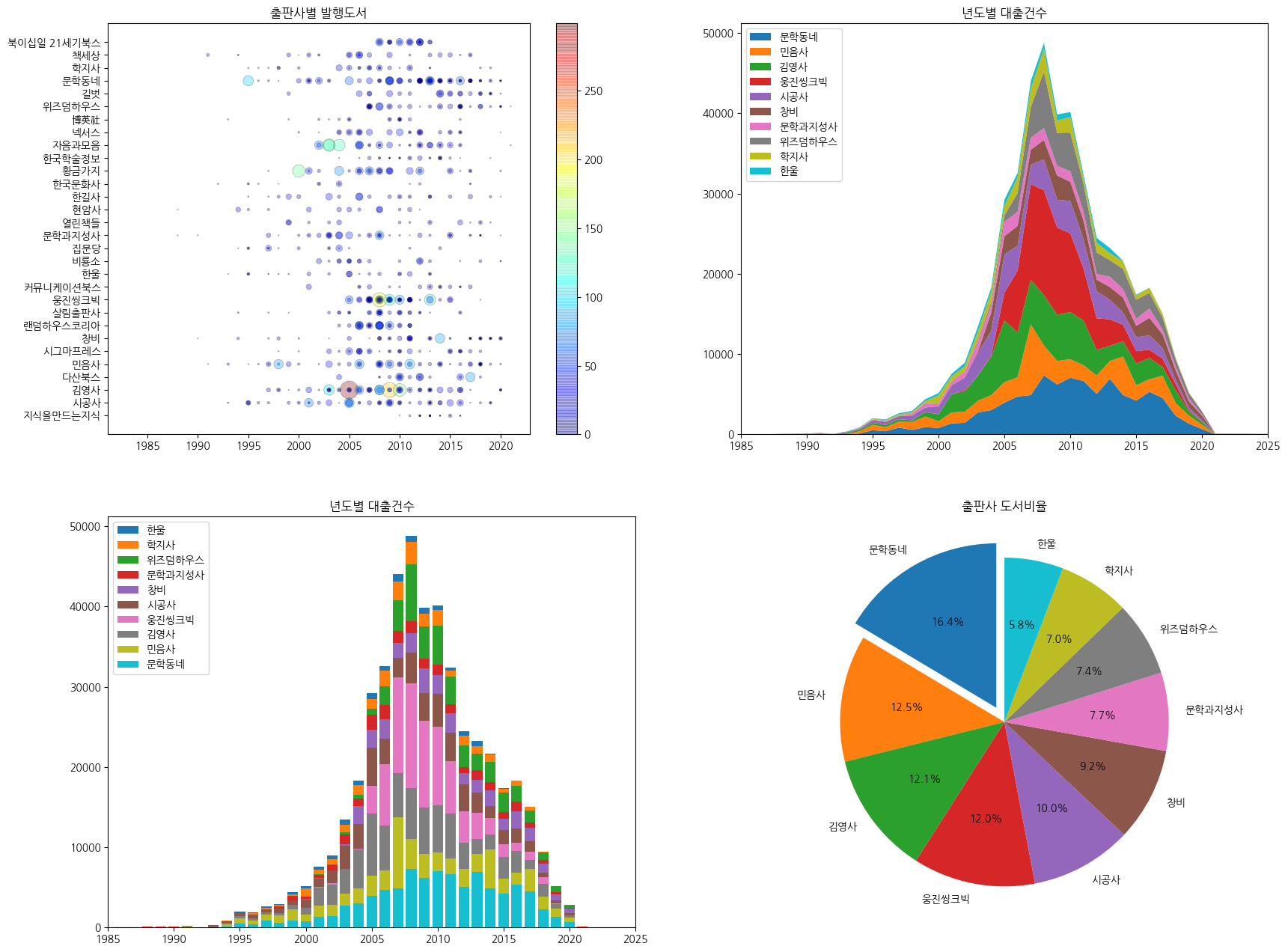
판다스로 여러개의 그래프 그리기
스택 영역 그래프 그리기 : plot.aera() 메서드
# 피벗 테이블 변환
ns_book11 = ns_book9.pivot_table(index='발행년도', columns='출판사', values='대출건수')
ns_book11.loc[2000:2005]

# 넘파이를 이용한 피벗 테이블 변환
import numpy as np
ns_book11 = ns_book7[top30_pubs_idx].pivot_table(
    index='발행년도', columns='출판사',
    values='대출건수', aggfunc=np.sum)
ns_book11.loc[2000:2005]

fig, ax = plt.subplots(figsize=(8, 6))
ns_book11[top10_pubs].plot.area(ax=ax, title='년도별 대출건수',
                                xlim=(1985, 2025))
ax.legend(loc='upper left')
fig.show()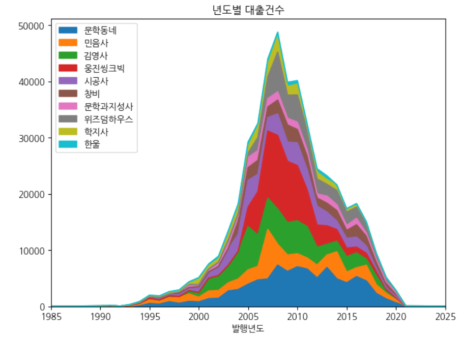
스택 막대 그래프 그리기 : plot.bar() 메서드
fig, ax = plt.subplots(figsize=(8, 6))
ns_book11.loc[1985:2025, top10_pubs].plot.bar(
    ax=ax, title='년도별 대출건수', width=0.8)
ax.legend(loc='upper left')
fig.show()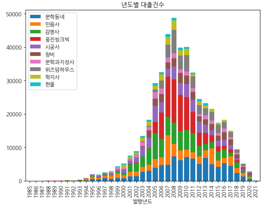
함수
| 함수 | 기능 |
|---|---|
| Axes.legend() | 그래프에 범례 추가 |
| Axes.set_xlim() | x축의 출력 범위 지정 |
| DataFrame.pivot_table() | 피벗 테이블 기능 제공 |
| Axes.stackplot() | 스택 영역 그래프 그리기 |
| DataFrame.plot.area() | 스택 영역 그래프 그리기 |
| DataFrame.plot.bar() | 막대 그래프 그리기 |
| DataFrame.cumsum() | 행이나 열 방향으로 누적 합을 계산 |
| Axes.pie() | 원 그래프 그리기 |
미션
- 기본 미션
- 선택 미션
위의 정리된 내용으로 대신하겠습니다.

업무하면서 쌓인 노하우를 정리하는 블로그🚀 풀스택 개발자를 지향하고 있습니다👻