Glass Bangle Defect Detection(다중 분류)
데이터 준비 : 드라이브 마운트 및 데이터 분리
# # 드라이브 마운트
# from google.colab import drive
# drive.mount('/content/drive')


# # 파일을 불러오기 위한 모듈
import os
# # 파일이 있는 경로로 이동
# %cd "/content/drive/MyDrive/deeplearning_project_ZB7"
# 경로 확인
os.getcwd()'c:\\Users\\theo\\Documents\\deep_learning\\dl-project'# 파일 확인
os.listdir()['best_model.h5',
'cnn_glass_bangle_defect_detection_epoch_15_with_adam_relu.h5',
'cnn_glass_bangle_defect_detection_epoch_30_with_adam_swish.h5',
'damaged_glass_bangle_classification.ipynb',
'dataset',
'dataset.zip',
'dataset_binary',
'image_classification_deeplearning_theo.ipynb',
'image_classification_model.h5',
'split_data',
'split_data_binary',
'theo_modified_binary.ipynb',
'theo_modified_categorical.ipynb',
'XAI_best_model.h5']!pip install split-foldersLooking in indexes: https://pypi.org/simple, https://us-python.pkg.dev/colab-wheels/public/simple/
Collecting split-folders
Downloading split_folders-0.5.1-py3-none-any.whl (8.4 kB)
Installing collected packages: split-folders
Successfully installed split-folders-0.5.1# 파일 나누기
import splitfolders
original_dir = 'dataset'
classes_list = os.listdir(original_dir)
base_dir = './split_data'
# os.mkdir(base_dir)
# splitfolders.ratio(original_dir, output=base_dir, seed = 35, ratio=(.8,.1,.1))# 원본 파일 확인
print('original/good :', len(os.listdir('dataset/good')))
print('original/broken :',len(os.listdir('dataset/broken')))
print('original/defect :',len(os.listdir('dataset/defect')))original/good : 520
original/broken : 316
original/defect : 244# train, validation, test로 나눠진 파일들 확인
print('train/good :', len(os.listdir('split_data/train/good')))
print('train/broken :',len(os.listdir('split_data/train/broken')))
print('train/defect :',len(os.listdir('split_data/train/defect')))
print('val/good :',len(os.listdir('split_data/val/good')))
print('val/broken :',len(os.listdir('split_data/val/broken')))
print('val/defect :',len(os.listdir('split_data/val/defect')))
print('test/good :',len(os.listdir('split_data/test/good')))
print('test/broken :',len(os.listdir('split_data/test/broken')))
print('test/defect :',len(os.listdir('split_data/test/defect')))train/good : 416
train/broken : 252
train/defect : 195
val/good : 52
val/broken : 31
val/defect : 24
test/good : 52
test/broken : 33
test/defect : 25데이터 준비 : 훈련 및 검증 데이터 경로 지정
# 경로 설정
train_dir = os.path.join(base_dir, 'train')
val_dir = os.path.join(base_dir, 'val')
test_dir = os.path.join(base_dir, 'test')
데이터 준비 : 이미지 데이터 전처리
# CUDA 적용 : 속도 이슈 해결
import torch

USE_CUDA = torch.cuda.is_available()
Device = torch.device('cuda' if USE_CUDA else 'cpu')

print(Device)cuda# 이미지 텐서화 작업
import torchvision.transforms as transforms
from torchvision.datasets import ImageFolder
transform_base = transforms.Compose([transforms.Resize((150,150)), transforms.ToTensor()])
train_dataset = ImageFolder(root='./split_data/train', transform=transform_base)
val_dataset = ImageFolder(root='./split_data/val', transform=transform_base)# 이미지 데이터 최종 전처리
from tensorflow.keras.preprocessing.image import ImageDataGenerator
train_datagen = ImageDataGenerator( rescale = 1.0/255.,
rotation_range=40,
width_shift_range=0.2,
height_shift_range=0.2,
shear_range=0.2,
zoom_range=0.2,
horizontal_flip=True,
fill_mode='nearest' )
test_datagen = ImageDataGenerator( rescale = 1.0/255. )
train_generator = train_datagen.flow_from_directory(train_dir,
batch_size=16,
class_mode='categorical',
target_size=(150, 150))
validation_generator = test_datagen.flow_from_directory(val_dir,
batch_size=16,
class_mode = 'categorical',
target_size = (150, 150))Found 863 images belonging to 3 classes.
Found 107 images belonging to 3 classes.모델 구성
# 모델 구성하기 : CNN
import tensorflow as tf


model = tf.keras.models.Sequential([
  tf.keras.layers.Conv2D(16, (3,3), activation='relu', input_shape=(150, 150, 3)),
  tf.keras.layers.MaxPooling2D(2,2),
  tf.keras.layers.Dropout(0.3),
  tf.keras.layers.Conv2D(32, (3,3), activation='relu'),
  tf.keras.layers.MaxPooling2D(2,2),
  tf.keras.layers.Dropout(0.3),
  tf.keras.layers.Conv2D(64, (3,3), activation='relu'),
  tf.keras.layers.MaxPooling2D(2,2),
  tf.keras.layers.Dropout(0.3),
  tf.keras.layers.Flatten(),
  tf.keras.layers.Dropout(0.3),
  tf.keras.layers.Dense(512, activation='relu'),
  tf.keras.layers.Dense(3, activation='softmax')
])

model.summary()
Model: "sequential"
_________________________________________________________________
Layer (type) Output Shape Param #
=================================================================
conv2d (Conv2D) (None, 148, 148, 16) 448
max_pooling2d (MaxPooling2D (None, 74, 74, 16) 0
)
dropout (Dropout) (None, 74, 74, 16) 0
conv2d_1 (Conv2D) (None, 72, 72, 32) 4640
max_pooling2d_1 (MaxPooling (None, 36, 36, 32) 0
2D)
dropout_1 (Dropout) (None, 36, 36, 32) 0
conv2d_2 (Conv2D) (None, 34, 34, 64) 18496
max_pooling2d_2 (MaxPooling (None, 17, 17, 64) 0
2D)
dropout_2 (Dropout) (None, 17, 17, 64) 0
flatten (Flatten) (None, 18496) 0
dropout_3 (Dropout) (None, 18496) 0
dense (Dense) (None, 512) 9470464
dense_1 (Dense) (None, 3) 1539
=================================================================
Total params: 9,495,587
Trainable params: 9,495,587
Non-trainable params: 0
_________________________________________________________________import tensorflow as tf
# 모델 컴파일하기
model.compile(optimizer=tf.keras.optimizers.Adam(learning_rate=0.001),
loss='categorical_crossentropy',
metrics=['accuracy'])from tensorflow.keras.callbacks import EarlyStopping, ModelCheckpoint
# 콜백 함수
es = EarlyStopping(monitor="val_loss", verbose=1, patience=10)
# 최적의 모델을 자동 저장
mc = ModelCheckpoint("best_model_ver2.h5", monitor='val_accuracy', save_best_only=True, verbose=1)# 모델 훈련하기
steps_per_epoch = 863 // 16
validation_steps = 107 // 16
hist = model.fit(train_generator,
validation_data=validation_generator,
steps_per_epoch=steps_per_epoch,
validation_steps=validation_steps,
epochs=50,
callbacks=[es, mc])Epoch 1/50
53/53 [==============================] - ETA: 0s - loss: 2.0033 - accuracy: 0.4286
Epoch 00001: val_accuracy improved from -inf to 0.50000, saving model to best_model_ver2.h5
53/53 [==============================] - 66s 1s/step - loss: 2.0033 - accuracy: 0.4286 - val_loss: 1.0479 - val_accuracy: 0.5000
Epoch 2/50
53/53 [==============================] - ETA: 0s - loss: 1.0603 - accuracy: 0.4829
Epoch 00002: val_accuracy improved from 0.50000 to 0.52083, saving model to best_model_ver2.h5
53/53 [==============================] - 69s 1s/step - loss: 1.0603 - accuracy: 0.4829 - val_loss: 1.0642 - val_accuracy: 0.5208
Epoch 3/50
53/53 [==============================] - ETA: 0s - loss: 1.0432 - accuracy: 0.4852
Epoch 00003: val_accuracy did not improve from 0.52083
53/53 [==============================] - 68s 1s/step - loss: 1.0432 - accuracy: 0.4852 - val_loss: 1.0636 - val_accuracy: 0.4479
Epoch 4/50
53/53 [==============================] - ETA: 0s - loss: 1.0223 - accuracy: 0.4829
Epoch 00004: val_accuracy did not improve from 0.52083
53/53 [==============================] - 63s 1s/step - loss: 1.0223 - accuracy: 0.4829 - val_loss: 0.9662 - val_accuracy: 0.5000
Epoch 5/50
53/53 [==============================] - ETA: 0s - loss: 0.9530 - accuracy: 0.4829
Epoch 00005: val_accuracy did not improve from 0.52083
53/53 [==============================] - 64s 1s/step - loss: 0.9530 - accuracy: 0.4829 - val_loss: 0.9644 - val_accuracy: 0.4688
Epoch 6/50
53/53 [==============================] - ETA: 0s - loss: 0.9420 - accuracy: 0.4829
Epoch 00006: val_accuracy did not improve from 0.52083
53/53 [==============================] - 66s 1s/step - loss: 0.9420 - accuracy: 0.4829 - val_loss: 0.9041 - val_accuracy: 0.4792
Epoch 7/50
53/53 [==============================] - ETA: 0s - loss: 0.9066 - accuracy: 0.5148
Epoch 00007: val_accuracy improved from 0.52083 to 0.55208, saving model to best_model_ver2.h5
53/53 [==============================] - 63s 1s/step - loss: 0.9066 - accuracy: 0.5148 - val_loss: 0.8260 - val_accuracy: 0.5521
Epoch 8/50
53/53 [==============================] - ETA: 0s - loss: 0.8881 - accuracy: 0.5762
Epoch 00008: val_accuracy improved from 0.55208 to 0.65625, saving model to best_model_ver2.h5
53/53 [==============================] - 59s 1s/step - loss: 0.8881 - accuracy: 0.5762 - val_loss: 0.7994 - val_accuracy: 0.6562
Epoch 9/50
53/53 [==============================] - ETA: 0s - loss: 0.8458 - accuracy: 0.5891
Epoch 00009: val_accuracy did not improve from 0.65625
53/53 [==============================] - 66s 1s/step - loss: 0.8458 - accuracy: 0.5891 - val_loss: 0.9232 - val_accuracy: 0.5833
Epoch 10/50
53/53 [==============================] - ETA: 0s - loss: 0.8501 - accuracy: 0.5773
Epoch 00010: val_accuracy did not improve from 0.65625
53/53 [==============================] - 59s 1s/step - loss: 0.8501 - accuracy: 0.5773 - val_loss: 0.7664 - val_accuracy: 0.6354
Epoch 11/50
53/53 [==============================] - ETA: 0s - loss: 0.8232 - accuracy: 0.5927
Epoch 00011: val_accuracy improved from 0.65625 to 0.69792, saving model to best_model_ver2.h5
53/53 [==============================] - 60s 1s/step - loss: 0.8232 - accuracy: 0.5927 - val_loss: 0.8101 - val_accuracy: 0.6979
Epoch 12/50
53/53 [==============================] - ETA: 0s - loss: 0.7685 - accuracy: 0.6387
Epoch 00012: val_accuracy did not improve from 0.69792
53/53 [==============================] - 64s 1s/step - loss: 0.7685 - accuracy: 0.6387 - val_loss: 0.7878 - val_accuracy: 0.6875
Epoch 13/50
53/53 [==============================] - ETA: 0s - loss: 0.7891 - accuracy: 0.6222
Epoch 00013: val_accuracy did not improve from 0.69792
53/53 [==============================] - 66s 1s/step - loss: 0.7891 - accuracy: 0.6222 - val_loss: 0.7527 - val_accuracy: 0.6979
Epoch 14/50
53/53 [==============================] - ETA: 0s - loss: 0.7829 - accuracy: 0.6234
Epoch 00014: val_accuracy improved from 0.69792 to 0.72917, saving model to best_model_ver2.h5
53/53 [==============================] - 65s 1s/step - loss: 0.7829 - accuracy: 0.6234 - val_loss: 0.7469 - val_accuracy: 0.7292
Epoch 15/50
53/53 [==============================] - ETA: 0s - loss: 0.7785 - accuracy: 0.6375
Epoch 00015: val_accuracy did not improve from 0.72917
53/53 [==============================] - 60s 1s/step - loss: 0.7785 - accuracy: 0.6375 - val_loss: 0.6510 - val_accuracy: 0.6771
Epoch 16/50
53/53 [==============================] - ETA: 0s - loss: 0.7712 - accuracy: 0.6411
Epoch 00016: val_accuracy did not improve from 0.72917
53/53 [==============================] - 66s 1s/step - loss: 0.7712 - accuracy: 0.6411 - val_loss: 0.7058 - val_accuracy: 0.6875
Epoch 17/50
53/53 [==============================] - ETA: 0s - loss: 0.7340 - accuracy: 0.6741
Epoch 00017: val_accuracy did not improve from 0.72917
53/53 [==============================] - 64s 1s/step - loss: 0.7340 - accuracy: 0.6741 - val_loss: 0.7103 - val_accuracy: 0.7188
Epoch 18/50
53/53 [==============================] - ETA: 0s - loss: 0.7129 - accuracy: 0.6647
Epoch 00018: val_accuracy did not improve from 0.72917
53/53 [==============================] - 81s 2s/step - loss: 0.7129 - accuracy: 0.6647 - val_loss: 0.6554 - val_accuracy: 0.6979
Epoch 19/50
53/53 [==============================] - ETA: 0s - loss: 0.7102 - accuracy: 0.6824
Epoch 00019: val_accuracy did not improve from 0.72917
53/53 [==============================] - 65s 1s/step - loss: 0.7102 - accuracy: 0.6824 - val_loss: 0.6315 - val_accuracy: 0.7292
Epoch 20/50
53/53 [==============================] - ETA: 0s - loss: 0.6891 - accuracy: 0.6812
Epoch 00020: val_accuracy improved from 0.72917 to 0.76042, saving model to best_model_ver2.h5
53/53 [==============================] - 66s 1s/step - loss: 0.6891 - accuracy: 0.6812 - val_loss: 0.6009 - val_accuracy: 0.7604
Epoch 21/50
53/53 [==============================] - ETA: 0s - loss: 0.6885 - accuracy: 0.6930
Epoch 00021: val_accuracy did not improve from 0.76042
53/53 [==============================] - 65s 1s/step - loss: 0.6885 - accuracy: 0.6930 - val_loss: 0.6705 - val_accuracy: 0.7604
Epoch 22/50
53/53 [==============================] - ETA: 0s - loss: 0.6889 - accuracy: 0.6978
Epoch 00022: val_accuracy did not improve from 0.76042
53/53 [==============================] - 64s 1s/step - loss: 0.6889 - accuracy: 0.6978 - val_loss: 0.6824 - val_accuracy: 0.7188
Epoch 23/50
53/53 [==============================] - ETA: 0s - loss: 0.6710 - accuracy: 0.6942
Epoch 00023: val_accuracy did not improve from 0.76042
53/53 [==============================] - 76s 1s/step - loss: 0.6710 - accuracy: 0.6942 - val_loss: 0.6926 - val_accuracy: 0.7500
Epoch 24/50
53/53 [==============================] - ETA: 0s - loss: 0.6687 - accuracy: 0.7131
Epoch 00024: val_accuracy did not improve from 0.76042
53/53 [==============================] - 66s 1s/step - loss: 0.6687 - accuracy: 0.7131 - val_loss: 0.5994 - val_accuracy: 0.7500
Epoch 25/50
53/53 [==============================] - ETA: 0s - loss: 0.6576 - accuracy: 0.6978
Epoch 00025: val_accuracy did not improve from 0.76042
53/53 [==============================] - 65s 1s/step - loss: 0.6576 - accuracy: 0.6978 - val_loss: 0.5757 - val_accuracy: 0.7604
Epoch 26/50
53/53 [==============================] - ETA: 0s - loss: 0.6198 - accuracy: 0.7332
Epoch 00026: val_accuracy did not improve from 0.76042
53/53 [==============================] - 64s 1s/step - loss: 0.6198 - accuracy: 0.7332 - val_loss: 0.6243 - val_accuracy: 0.7604
Epoch 27/50
53/53 [==============================] - ETA: 0s - loss: 0.6114 - accuracy: 0.7379
Epoch 00027: val_accuracy improved from 0.76042 to 0.78125, saving model to best_model_ver2.h5
53/53 [==============================] - 68s 1s/step - loss: 0.6114 - accuracy: 0.7379 - val_loss: 0.6073 - val_accuracy: 0.7812
Epoch 28/50
53/53 [==============================] - ETA: 0s - loss: 0.6087 - accuracy: 0.7438
Epoch 00028: val_accuracy did not improve from 0.78125
53/53 [==============================] - 61s 1s/step - loss: 0.6087 - accuracy: 0.7438 - val_loss: 0.6410 - val_accuracy: 0.7188
Epoch 29/50
53/53 [==============================] - ETA: 0s - loss: 0.5982 - accuracy: 0.7344
Epoch 00029: val_accuracy did not improve from 0.78125
53/53 [==============================] - 62s 1s/step - loss: 0.5982 - accuracy: 0.7344 - val_loss: 0.6185 - val_accuracy: 0.7396
Epoch 30/50
53/53 [==============================] - ETA: 0s - loss: 0.5970 - accuracy: 0.7414
Epoch 00030: val_accuracy improved from 0.78125 to 0.79167, saving model to best_model_ver2.h5
53/53 [==============================] - 77s 1s/step - loss: 0.5970 - accuracy: 0.7414 - val_loss: 0.5157 - val_accuracy: 0.7917
Epoch 31/50
53/53 [==============================] - ETA: 0s - loss: 0.5670 - accuracy: 0.7615
Epoch 00031: val_accuracy did not improve from 0.79167
53/53 [==============================] - 62s 1s/step - loss: 0.5670 - accuracy: 0.7615 - val_loss: 0.6940 - val_accuracy: 0.6979
Epoch 32/50
53/53 [==============================] - ETA: 0s - loss: 0.5873 - accuracy: 0.7426
Epoch 00032: val_accuracy did not improve from 0.79167
53/53 [==============================] - 63s 1s/step - loss: 0.5873 - accuracy: 0.7426 - val_loss: 0.6442 - val_accuracy: 0.7604
Epoch 33/50
53/53 [==============================] - ETA: 0s - loss: 0.5943 - accuracy: 0.7473
Epoch 00033: val_accuracy did not improve from 0.79167
53/53 [==============================] - 65s 1s/step - loss: 0.5943 - accuracy: 0.7473 - val_loss: 0.6518 - val_accuracy: 0.7396
Epoch 34/50
53/53 [==============================] - ETA: 0s - loss: 0.5622 - accuracy: 0.7544
Epoch 00034: val_accuracy did not improve from 0.79167
53/53 [==============================] - 62s 1s/step - loss: 0.5622 - accuracy: 0.7544 - val_loss: 0.5884 - val_accuracy: 0.7604
Epoch 35/50
53/53 [==============================] - ETA: 0s - loss: 0.5723 - accuracy: 0.7580
Epoch 00035: val_accuracy did not improve from 0.79167
53/53 [==============================] - 62s 1s/step - loss: 0.5723 - accuracy: 0.7580 - val_loss: 0.5645 - val_accuracy: 0.7708
Epoch 36/50
53/53 [==============================] - ETA: 0s - loss: 0.5876 - accuracy: 0.7591
Epoch 00036: val_accuracy did not improve from 0.79167
53/53 [==============================] - 62s 1s/step - loss: 0.5876 - accuracy: 0.7591 - val_loss: 0.5993 - val_accuracy: 0.7812
Epoch 37/50
53/53 [==============================] - ETA: 0s - loss: 0.5560 - accuracy: 0.7485
Epoch 00037: val_accuracy improved from 0.79167 to 0.81250, saving model to best_model_ver2.h5
53/53 [==============================] - 63s 1s/step - loss: 0.5560 - accuracy: 0.7485 - val_loss: 0.5231 - val_accuracy: 0.8125
Epoch 38/50
53/53 [==============================] - ETA: 0s - loss: 0.5336 - accuracy: 0.7686
Epoch 00038: val_accuracy did not improve from 0.81250
53/53 [==============================] - 64s 1s/step - loss: 0.5336 - accuracy: 0.7686 - val_loss: 0.5278 - val_accuracy: 0.7917
Epoch 39/50
53/53 [==============================] - ETA: 0s - loss: 0.5490 - accuracy: 0.7780
Epoch 00039: val_accuracy did not improve from 0.81250
53/53 [==============================] - 64s 1s/step - loss: 0.5490 - accuracy: 0.7780 - val_loss: 0.5184 - val_accuracy: 0.8021
Epoch 40/50
53/53 [==============================] - ETA: 0s - loss: 0.5622 - accuracy: 0.7580
Epoch 00040: val_accuracy did not improve from 0.81250
53/53 [==============================] - 64s 1s/step - loss: 0.5622 - accuracy: 0.7580 - val_loss: 0.5510 - val_accuracy: 0.7500
Epoch 00040: early stopping# 반복학습을 피하기 위한 모델 리셋용
tf.keras.backend.clear_session()모델 검증
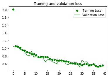
import matplotlib.pyplot as plt

acc = hist.history['accuracy']
val_acc = hist.history['val_accuracy']
loss = hist.history['loss']
val_loss = hist.history['val_loss']

epochs = range(len(acc))

plt.plot(epochs, acc, 'bo', label='Training accuracy')
plt.plot(epochs, val_acc, 'b', label='Validation accuracy')
plt.title('Training and validation accuracy')
plt.legend()

plt.figure()

plt.plot(epochs, loss, 'go', label='Training Loss')
plt.plot(epochs, val_loss, 'g', label='Validation Loss')
plt.title('Training and validation loss')
plt.legend()

plt.show()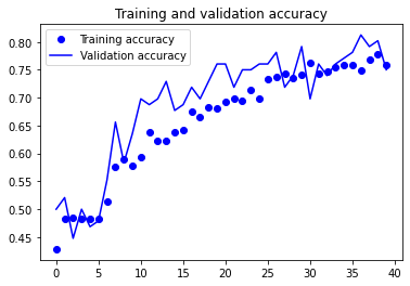
# 수치 비교
plt.figure(figsize=(12,6))
plt.plot(acc, label = 'acc')
plt.plot(val_acc, label = 'val_acc')
plt.plot(loss, label = 'loss')
plt.plot(val_loss, label = 'val_loss')
plt.legend()
plt.show()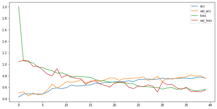
from keras.models import load_model

# 모델 불러오기
model = load_model('best_model_ver2.h5')
모델 평가
# 테스트 데이터 전처리
test_datagen  = ImageDataGenerator( rescale = 1.0/255. )

test_generator =  test_datagen.flow_from_directory(test_dir,
                                                  batch_size = 16,
                                                  class_mode  = 'categorical',
                                                  target_size = (150, 150))
scores = model.evaluate(test_generator, steps = 110 // 16)
print('%s : %.2f%%'%(model.metrics_names[1], scores[1]*100))6/6 [==============================] - 7s 1s/step - loss: 0.5925 - accuracy: 0.7500
accuracy : 75.00%모델 준비 완료 --> saliency 적용
!pip install saliencyLooking in indexes: https://pypi.org/simple, https://us-python.pkg.dev/colab-wheels/public/simple/
Collecting saliency
Downloading saliency-0.2.0-py2.py3-none-any.whl (86 kB)
[2K [90m━━━━━━━━━━━━━━━━━━━━━━━━━━━━━━━━━━━━━━━━[0m [32m86.2/86.2 KB[0m [31m3.0 MB/s[0m eta [36m0:00:00[0m
[?25hRequirement already satisfied: scikit-image in /usr/local/lib/python3.8/dist-packages (from saliency) (0.18.3)
Requirement already satisfied: numpy in /usr/local/lib/python3.8/dist-packages (from saliency) (1.21.6)
Requirement already satisfied: scipy>=1.0.1 in /usr/local/lib/python3.8/dist-packages (from scikit-image->saliency) (1.7.3)
Requirement already satisfied: networkx>=2.0 in /usr/local/lib/python3.8/dist-packages (from scikit-image->saliency) (3.0)
Requirement already satisfied: matplotlib!=3.0.0,>=2.0.0 in /usr/local/lib/python3.8/dist-packages (from scikit-image->saliency) (3.2.2)
Requirement already satisfied: pillow!=7.1.0,!=7.1.1,>=4.3.0 in /usr/local/lib/python3.8/dist-packages (from scikit-image->saliency) (7.1.2)
Requirement already satisfied: PyWavelets>=1.1.1 in /usr/local/lib/python3.8/dist-packages (from scikit-image->saliency) (1.4.1)
Requirement already satisfied: imageio>=2.3.0 in /usr/local/lib/python3.8/dist-packages (from scikit-image->saliency) (2.9.0)
Requirement already satisfied: tifffile>=2019.7.26 in /usr/local/lib/python3.8/dist-packages (from scikit-image->saliency) (2023.2.3)
Requirement already satisfied: python-dateutil>=2.1 in /usr/local/lib/python3.8/dist-packages (from matplotlib!=3.0.0,>=2.0.0->scikit-image->saliency) (2.8.2)
Requirement already satisfied: cycler>=0.10 in /usr/local/lib/python3.8/dist-packages (from matplotlib!=3.0.0,>=2.0.0->scikit-image->saliency) (0.11.0)
Requirement already satisfied: pyparsing!=2.0.4,!=2.1.2,!=2.1.6,>=2.0.1 in /usr/local/lib/python3.8/dist-packages (from matplotlib!=3.0.0,>=2.0.0->scikit-image->saliency) (3.0.9)
Requirement already satisfied: kiwisolver>=1.0.1 in /usr/local/lib/python3.8/dist-packages (from matplotlib!=3.0.0,>=2.0.0->scikit-image->saliency) (1.4.4)
Requirement already satisfied: six>=1.5 in /usr/local/lib/python3.8/dist-packages (from python-dateutil>=2.1->matplotlib!=3.0.0,>=2.0.0->scikit-image->saliency) (1.15.0)
Installing collected packages: saliency
Successfully installed saliency-0.2.0Saliency 모델의 output과 input 사이의 gradient 연산 처리
import saliency.core as saliency
import tensorflow as tf
import numpy as np

def model_fn(images, call_model_args, expected_keys=None):

    target_class_idx = call_model_args['class']
    model = call_model_args['model']
    images = tf.convert_to_tensor(images)

    with tf.GradientTape() as tape:
        if expected_keys==[saliency.base.INPUT_OUTPUT_GRADIENTS]:
            tape.watch(images)
            output = model(images)
            output = output[:,target_class_idx]
            gradients = np.array(tape.gradient(output, images))
            return {saliency.base.INPUT_OUTPUT_GRADIENTS: gradients}
        else:
            conv, output = model(images)
            gradients = np.array(tape.gradient(output, conv))
            return {saliency.base.CONVOLUTION_LAYER_VALUES: conv,
                    saliency.base.CONVOLUTION_OUTPUT_GRADIENTS: gradients}
Saliency map을 이용하여 기여도 맵 추출 함수
def vanilla_saliency(model, img):
    """
    :model: 학습된 인공지능 모델
            인공지능 모델이 바뀔 때, 기여도 맵 또한 변경됨.
    :img:   기여도 맵을 추출하고 하는 이미지 데이터
    :return: 추출된 기여도 맵

    """
    pred = model(np.array([img]))
    pred_cls = np.argmax(pred[0])
    args = {'model': model, 'class': pred_cls}

    grad = saliency.GradientSaliency()
    attr = grad.GetMask(img, model_fn, args)
    attr = saliency.VisualizeImageGrayscale(attr)

    return tf.reshape(attr, (*attr.shape, 1))

def ig(model, img):
    pred = model(np.array([img]))
    pred_cls = np.argmax(pred[0])
    args = {'model': model, 'class': pred_cls}

    baseline = np.zeros(img.shape)
    ig = saliency.IntegratedGradients()
    attr = ig.GetMask(img, model_fn, args, x_steps=25, x_baseline=baseline, batch_size=20)
    attr = saliency.VisualizeImageGrayscale(attr)

    return tf.reshape(attr, (*attr.shape, 1))

def smooth_saliency(model, img):
    pred = model(np.array([img]))
    pred_cls = np.argmax(pred[0])
    args = {'model': model, 'class': pred_cls}

    smooth_grad = saliency.GradientSaliency()
    smooth_attr = smooth_grad.GetSmoothedMask(img, model_fn, args)
    smooth_attr = saliency.VisualizeImageGrayscale(smooth_attr)

    return tf.reshape(smooth_attr, (*smooth_attr.shape, 1))

def smooth_ig(model, img):

    pred = model(np.array([img]))
    pred_cls = np.argmax(pred[0])
    args = {'model': model, 'class': pred_cls}

    baseline = np.zeros(img.shape)
    smooth_ig = saliency.IntegratedGradients()

    smooth_attr = smooth_ig.GetSmoothedMask(
        img, model_fn, args, x_steps=25, x_baseline=baseline, batch_size=20)

    smooth_attr = saliency.VisualizeImageGrayscale(smooth_attr)

    return tf.reshape(smooth_attr, (*smooth_attr.shape, 1))
sample data 시각화: 분류 라벨별('good' or 'broken' or 'defect')
# sample data 시각화 : broken 이미지

import matplotlib.pyplot as plt

plt.imshow(x_val[4])<matplotlib.image.AxesImage at 0x148b6db8af0>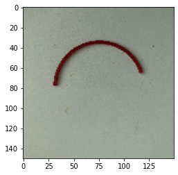
sample_image = x_val[4]
sample_saliency_xai_image = vanilla_saliency(model, x_val[4])
sample_ig_xai_image = ig(model, x_val[4])plt.figure(figsize=(15, 5))
plt.subplot(1, 3, 1)
plt.imshow(np.reshape(sample_image, (150, 150, 3)))
plt.title("origin image")
plt.axis('off')
plt.subplot(1, 3, 2)
plt.imshow(np.reshape(sample_saliency_xai_image, (150, 150)))
plt.title("saliency image")
plt.axis('off')
plt.subplot(1, 3, 3)
plt.imshow(np.reshape(sample_ig_xai_image, (150, 150)))
plt.title("ig image")
plt.axis('off')
plt.show()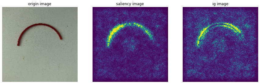
# sample data 시각화 : defect 이미지

plt.imshow(x_val[13])<matplotlib.image.AxesImage at 0x148800d65b0>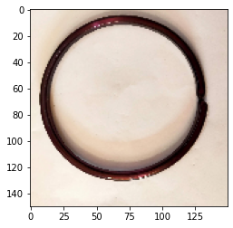
sample_image = x_val[13]
sample_saliency_xai_image = vanilla_saliency(model, x_val[13])
sample_ig_xai_image = ig(model, x_val[13])plt.figure(figsize=(15, 5))
plt.subplot(1, 3, 1)
plt.imshow(np.reshape(sample_image, (150, 150, 3)))
plt.title("origin image")
plt.axis('off')
plt.subplot(1, 3, 2)
plt.imshow(np.reshape(sample_saliency_xai_image, (150, 150)))
plt.title("saliency image")
plt.axis('off')
plt.subplot(1, 3, 3)
plt.imshow(np.reshape(sample_ig_xai_image, (150, 150)))
plt.title("ig image")
plt.axis('off')
plt.show()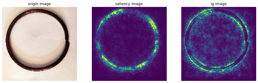
# sample data 시각화 : good 이미지

plt.imshow(x_val[21])<matplotlib.image.AxesImage at 0x148b9d09310>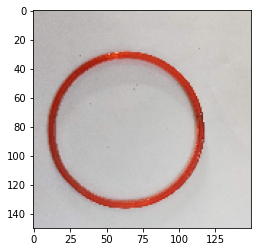
sample_image = x_val[21]
sample_saliency_xai_image = vanilla_saliency(model, x_val[21])
sample_ig_xai_image = ig(model, x_val[21])plt.figure(figsize=(15, 5))
plt.subplot(1, 3, 1)
plt.imshow(np.reshape(sample_image, (150, 150, 3)))
plt.title("origin image")
plt.axis('off')
plt.subplot(1, 3, 2)
plt.imshow(np.reshape(sample_saliency_xai_image, (150, 150)))
plt.title("saliency image")
plt.axis('off')
plt.subplot(1, 3, 3)
plt.imshow(np.reshape(sample_ig_xai_image, (150, 150)))
plt.title("ig image")
plt.axis('off')
plt.show()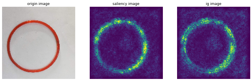
XAI형태로 데이터 추출
- validation_generator, train_generator 안에 있는 모든 데이터들을 이어서 학습
- 모든 데이터를 잇는 방식은 batch로 처리하는 방식에 비해서 속도 측면에서 비효율적
- 따라서 모델을 상정하고 generator에서 batch를 반복적으로 추출
- 각각의 batch를 차례대로 ig 처리해서 model에 순차적으로 학습
# 두 데이터 모두 batch size를 16개로 다시 전처리

train_datagen = ImageDataGenerator( rescale = 1.0/255. )


train_generator = train_datagen.flow_from_directory(train_dir,
                                                  batch_size=16,
                                                  class_mode='categorical',
                                                  target_size=(150, 150))
validation_generator =  train_datagen.flow_from_directory(val_dir,
                                                       batch_size=16,
                                                       class_mode  = 'categorical',
                                                       target_size = (150, 150))

test_generator =  train_datagen.flow_from_directory(test_dir,
                                                       batch_size=16,
                                                       class_mode  = 'categorical',
                                                       target_size = (150, 150))
Found 863 images belonging to 3 classes.
Found 107 images belonging to 3 classes.
Found 110 images belonging to 3 classes.iterators_1 = iter(train_generator)
iterators_2 = iter(validation_generator)
iterators_3 = iter(test_generator)
cnt = 0
while True:
x, y = next(iterators_1)
z = len(x)
cnt += 1
if cnt == 1:
X_train = x
y_train = y
else:
X_train = np.concatenate((X_train, x), axis=0)
y_train = np.concatenate((y_train, y), axis=0)
if z == 863 % 16:
break
while True:
x, y = next(iterators_2)
z = len(x)
X_train = np.concatenate((X_train, x), axis=0)
y_train = np.concatenate((y_train, y), axis=0)
if z == 107 % 16:
break
cnt = 0
while True:
x, y = next(iterators_3)
z = len(x)
cnt += 1
if cnt == 1:
X_val = x
y_val = y
else:
X_val = np.concatenate((X_val, x), axis=0)
y_val = np.concatenate((y_val, y), axis=0)
if z == 110 % 16:
break
ig_x_train = np.zeros_like(X_train)
ig_x_test = np.zeros_like(X_val)
for i in range(len(ig_x_train)):
ig_x_train[i] = ig(model, X_train[i])
for i in range(len(ig_x_test)):
ig_x_test[i] = ig(model, X_val[i])XAI 추출 데이터 모델 생성
new_model = tf.keras.models.Sequential([
  tf.keras.layers.Conv2D(16, (3,3), activation='relu', input_shape=(150, 150, 3)),
  tf.keras.layers.MaxPooling2D(2,2),
  tf.keras.layers.Dropout(0.3),
  tf.keras.layers.Conv2D(32, (3,3), activation='relu'),
  tf.keras.layers.MaxPooling2D(2,2),
  tf.keras.layers.Dropout(0.3),
  tf.keras.layers.Conv2D(64, (3,3), activation='relu'),
  tf.keras.layers.MaxPooling2D(2,2),
  tf.keras.layers.Dropout(0.3),
  tf.keras.layers.Flatten(),
  tf.keras.layers.Dropout(0.3),
  tf.keras.layers.Dense(512, activation='relu'),
  tf.keras.layers.Dense(3, activation='softmax')
])

new_model.compile(optimizer=tf.keras.optimizers.Adam(learning_rate=0.001),
                  loss='categorical_crossentropy',
                  metrics = ['accuracy'])

new_model.fit(ig_x_train, y_train, epochs=30, shuffle=True)
Epoch 1/30
31/31 [==============================] - 6s 144ms/step - loss: 0.9805 - accuracy: 0.5567
Epoch 2/30
31/31 [==============================] - 4s 127ms/step - loss: 0.7443 - accuracy: 0.6897
Epoch 3/30
31/31 [==============================] - 4s 128ms/step - loss: 0.6146 - accuracy: 0.7443
Epoch 4/30
31/31 [==============================] - 4s 127ms/step - loss: 0.5413 - accuracy: 0.7814
Epoch 5/30
31/31 [==============================] - 4s 128ms/step - loss: 0.4548 - accuracy: 0.8175
Epoch 6/30
31/31 [==============================] - 4s 127ms/step - loss: 0.3890 - accuracy: 0.8402
Epoch 7/30
31/31 [==============================] - 4s 128ms/step - loss: 0.3484 - accuracy: 0.8577
Epoch 8/30
31/31 [==============================] - 4s 127ms/step - loss: 0.3066 - accuracy: 0.8732
Epoch 9/30
31/31 [==============================] - 4s 127ms/step - loss: 0.2545 - accuracy: 0.9010
Epoch 10/30
31/31 [==============================] - 4s 127ms/step - loss: 0.1987 - accuracy: 0.9206
Epoch 11/30
31/31 [==============================] - 4s 127ms/step - loss: 0.1738 - accuracy: 0.9351
Epoch 12/30
31/31 [==============================] - 4s 131ms/step - loss: 0.1562 - accuracy: 0.9464
Epoch 13/30
31/31 [==============================] - 4s 131ms/step - loss: 0.1629 - accuracy: 0.9330
Epoch 14/30
31/31 [==============================] - 4s 135ms/step - loss: 0.1036 - accuracy: 0.9619
Epoch 15/30
31/31 [==============================] - 4s 128ms/step - loss: 0.0715 - accuracy: 0.9732
Epoch 16/30
31/31 [==============================] - 4s 130ms/step - loss: 0.0780 - accuracy: 0.9732
Epoch 17/30
31/31 [==============================] - 4s 129ms/step - loss: 0.0854 - accuracy: 0.9691
Epoch 18/30
31/31 [==============================] - 4s 139ms/step - loss: 0.0723 - accuracy: 0.9732
Epoch 19/30
31/31 [==============================] - 4s 129ms/step - loss: 0.0590 - accuracy: 0.9794
Epoch 20/30
31/31 [==============================] - 4s 127ms/step - loss: 0.0505 - accuracy: 0.9835
Epoch 21/30
31/31 [==============================] - 4s 128ms/step - loss: 0.0350 - accuracy: 0.9897
Epoch 22/30
31/31 [==============================] - 4s 128ms/step - loss: 0.0561 - accuracy: 0.9732
Epoch 23/30
31/31 [==============================] - 4s 128ms/step - loss: 0.0644 - accuracy: 0.9753
Epoch 24/30
31/31 [==============================] - 4s 128ms/step - loss: 0.0445 - accuracy: 0.9866
Epoch 25/30
31/31 [==============================] - 4s 130ms/step - loss: 0.0311 - accuracy: 0.9907
Epoch 26/30
31/31 [==============================] - 4s 128ms/step - loss: 0.0417 - accuracy: 0.9876
Epoch 27/30
31/31 [==============================] - 4s 129ms/step - loss: 0.0215 - accuracy: 0.9928
Epoch 28/30
31/31 [==============================] - 4s 128ms/step - loss: 0.0245 - accuracy: 0.9907
Epoch 29/30
31/31 [==============================] - 4s 128ms/step - loss: 0.0302 - accuracy: 0.9918
Epoch 30/30
31/31 [==============================] - 4s 129ms/step - loss: 0.0246 - accuracy: 0.9918
<keras.callbacks.History at 0x2063d3a5a00>plt.imshow(X_val[0])<matplotlib.image.AxesImage at 0x1e8014ee250>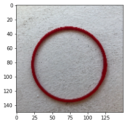
plt.imshow(ig_x_test[0])<matplotlib.image.AxesImage at 0x1e8014893d0>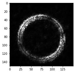
# 모델 불러오기

new_model = load_model('XAI_best_model.h5')
예측이 틀린 데이터 추출
# x, y = next(iter(test_generator)) # next를 실행하면 다시 shuffle 됨
print(ig_x_test[0].shape,len(ig_x_test))

predictions = new_model.predict(ig_x_test)
predictions = np.round(predictions).astype('float')

# 틀린 친구들의 인덱스 도출
# incorrect_idx = np.where(predictions != y_val)[0]
# print('예측 틀린 데이터 수 : ',len(incorrect_idx))

incorrect_idx = []

for i in range(len(ig_x_test)):
    cnt = 0
    while cnt < 3:
        if predictions[i][cnt] == 1:
            predictions_idx = cnt
        if y_val[i][cnt] == 1:
            y_val_idx = cnt
        cnt += 1

    if predictions_idx != y_val_idx:
        incorrect_idx.append(i)

print('예측 틀린 데이터 수 : ',len(incorrect_idx))
print('테스트 성능 : ', (110 - len(incorrect_idx)) / 110 * 100)
(150, 150, 3) 110
예측 틀린 데이터 수 : 29
테스트 성능 : 73.63636363636363# 틀린 데이터 이미지와 레이블을 가지고 오기
incorrect_images = []
incorrect_labels = []
correct_labels=[]
for i in incorrect_idx:
incorrect_images.append(X_val[i])
incorrect_labels.append(predictions[i])
correct_labels.append(y_val[i])
incorrect_images = np.array(incorrect_images)
incorrect_labels = np.array(incorrect_labels)
correct_labels = np.array(correct_labels)# 틀린 데이터 이미지 조회
for i, (img, label) in enumerate(zip(incorrect_images, incorrect_labels)):
plt.subplot(2, 9, i + 1)
plt.imshow(img)
plt.axis("off")
if label == 1:
plt.title("Label: Broken")
else:
plt.title("Label: Good")
plt.tight_layout()
plt.show()---------------------------------------------------------------------------
ValueError Traceback (most recent call last)
<ipython-input-250-332f48cd2ebc> in <module>
5 plt.imshow(img)
6 plt.axis("off")
----> 7 if label == 1:
8 plt.title("Label: Broken")
9 else:
ValueError: The truth value of an array with more than one element is ambiguous. Use a.any() or a.all()
XAI: LIME
pip install limeCollecting lime
Downloading lime-0.2.0.1.tar.gz (275 kB)
-------------------------------------- 275.7/275.7 kB 8.6 MB/s eta 0:00:00
Preparing metadata (setup.py): started
Preparing metadata (setup.py): finished with status 'done'
Note: you may need to restart the kernel to use updated packages.Requirement already satisfied: matplotlib in c:\users\theo\miniconda3\envs\ds_study\lib\site-packages (from lime) (3.5.2)
Requirement already satisfied: numpy in c:\users\theo\appdata\roaming\python\python38\site-packages (from lime) (1.24.2)
Requirement already satisfied: scipy in c:\users\theo\miniconda3\envs\ds_study\lib\site-packages (from lime) (1.10.0)
Requirement already satisfied: tqdm in c:\users\theo\miniconda3\envs\ds_study\lib\site-packages (from lime) (4.64.1)
Requirement already satisfied: scikit-learn>=0.18 in c:\users\theo\miniconda3\envs\ds_study\lib\site-packages (from lime) (1.1.3)
WARNING: Ignoring invalid distribution -illow (c:\users\theo\miniconda3\envs\ds_study\lib\site-packages)
WARNING: Ignoring invalid distribution -illow (c:\users\theo\miniconda3\envs\ds_study\lib\site-packages)
WARNING: Ignoring invalid distribution -illow (c:\users\theo\miniconda3\envs\ds_study\lib\site-packages)
WARNING: Error parsing requirements for markupsafe: [Errno 2] No such file or directory: 'c:\\users\\theo\\miniconda3\\envs\\ds_study\\lib\\site-packages\\MarkupSafe-2.1.1.dist-info\\METADATA'
WARNING: Ignoring invalid distribution -illow (c:\users\theo\miniconda3\envs\ds_study\lib\site-packages)
WARNING: Ignoring invalid distribution -illow (c:\users\theo\miniconda3\envs\ds_study\lib\site-packages)
WARNING: Ignoring invalid distribution -illow (c:\users\theo\miniconda3\envs\ds_study\lib\site-packages)
WARNING: Ignoring invalid distribution -illow (c:\users\theo\miniconda3\envs\ds_study\lib\site-packages)
Requirement already satisfied: scikit-image>=0.12 in c:\users\theo\miniconda3\envs\ds_study\lib\site-packages (from lime) (0.19.3)
Requirement already satisfied: packaging>=20.0 in c:\users\theo\miniconda3\envs\ds_study\lib\site-packages (from scikit-image>=0.12->lime) (22.0)
Requirement already satisfied: tifffile>=2019.7.26 in c:\users\theo\miniconda3\envs\ds_study\lib\site-packages (from scikit-image>=0.12->lime) (2023.2.3)
Requirement already satisfied: imageio>=2.4.1 in c:\users\theo\miniconda3\envs\ds_study\lib\site-packages (from scikit-image>=0.12->lime) (2.25.1)
Requirement already satisfied: PyWavelets>=1.1.1 in c:\users\theo\miniconda3\envs\ds_study\lib\site-packages (from scikit-image>=0.12->lime) (1.4.1)
Requirement already satisfied: pillow!=7.1.0,!=7.1.1,!=8.3.0,>=6.1.0 in c:\users\theo\appdata\roaming\python\python38\site-packages (from scikit-image>=0.12->lime) (9.4.0)
Requirement already satisfied: networkx>=2.2 in c:\users\theo\miniconda3\envs\ds_study\lib\site-packages (from scikit-image>=0.12->lime) (3.0)
Requirement already satisfied: threadpoolctl>=2.0.0 in c:\users\theo\miniconda3\envs\ds_study\lib\site-packages (from scikit-learn>=0.18->lime) (2.2.0)
Requirement already satisfied: joblib>=1.0.0 in c:\users\theo\miniconda3\envs\ds_study\lib\site-packages (from scikit-learn>=0.18->lime) (1.2.0)
Requirement already satisfied: kiwisolver>=1.0.1 in c:\users\theo\miniconda3\envs\ds_study\lib\site-packages (from matplotlib->lime) (1.4.4)
Requirement already satisfied: python-dateutil>=2.7 in c:\users\theo\appdata\roaming\python\python38\site-packages (from matplotlib->lime) (2.8.1)
Requirement already satisfied: pyparsing>=2.2.1 in c:\users\theo\appdata\roaming\python\python38\site-packages (from matplotlib->lime) (2.4.7)
Requirement already satisfied: cycler>=0.10 in c:\users\theo\miniconda3\envs\ds_study\lib\site-packages (from matplotlib->lime) (0.11.0)
Requirement already satisfied: fonttools>=4.22.0 in c:\users\theo\miniconda3\envs\ds_study\lib\site-packages (from matplotlib->lime) (4.25.0)
Requirement already satisfied: colorama in c:\users\theo\appdata\roaming\python\python38\site-packages (from tqdm->lime) (0.4.3)
Requirement already satisfied: six>=1.5 in c:\users\theo\appdata\roaming\python\python38\site-packages (from python-dateutil>=2.7->matplotlib->lime) (1.14.0)
Building wheels for collected packages: lime
Building wheel for lime (setup.py): started
Building wheel for lime (setup.py): finished with status 'done'
Created wheel for lime: filename=lime-0.2.0.1-py3-none-any.whl size=283839 sha256=77181b2177b58b887de195ce0cd657cc0747fc013d0fe1e10679204fc8f492fc
Stored in directory: c:\users\theo\appdata\local\pip\cache\wheels\ef\f5\11\572c4d43760b43708e7ddb4b401a01742dcb4299a0aa385023
Successfully built lime
Installing collected packages: lime
Successfully installed lime-0.2.0.1from lime import lime_image
from lime.wrappers.scikit_image import SegmentationAlgorithm
explainer = lime_image.LimeImageExplainer()# 이미지를 슈퍼픽셀로 분할하는 알고리즘 설정
# quickshift, slic, felzenswalb 등이 존재
segmenter = SegmentationAlgorithm('slic',
n_segments=100, # 이미지 분할 조각 개수
compactnes=1, # 유사한 파트를 합치는 함수
sigma=1) # 스무딩 역할: 0과 1사이의 floatolivetti_test_index = 0
X_test, y_test = next(iter(test_generator))
exp = explainer.explain_instance(X_test[olivetti_test_index],
classifier_fn=model.predict, # 40개 class 확률 반환
top_labels=1, # 확률 기준 1~5위
num_samples=1000, # sample space
segmentation_fn=segmenter) # 분할 알고리즘 0%| | 0/1000 [00:00<?, ?it/s]# sklearn의 regressor 기본 설명 모델로 사용
from skimage.color import label2rgb
y_test_num = b
# 캔버스
fig, ((ax1, ax2), (ax3, ax4)) = plt.subplots(2, 2, figsize=(8, 8))
ax = [ax1, ax2, ax3, ax4]
for i in ax:
i.grid(False)
# 모든 세그먼트 출력
temp, mask = exp.get_image_and_mask(y_test_num[0],
positive_only=False, # 설명 모델이 결과값을 가장 잘 설명하는 이미지 영역만 출력
num_features=8, # 분할 영역의 크기
hide_rest=False) # 이미지를 분류하는 데 도움이 되는 서브모듈 외의 모듈도 출력
# 이미지만 출력
ax3.imshow(temp, interpolation='nearest')
ax3.set_title('Show output image only')
Text(0.5, 1.0, 'Show mask only')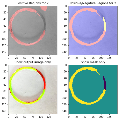
XAI: Grad-CAM
!pip install grad-camCollecting grad-cam
Downloading grad-cam-1.4.6.tar.gz (7.8 MB)
---------------------------------------- 7.8/7.8 MB 33.2 MB/s eta 0:00:00
Installing build dependencies: started
Installing build dependencies: finished with status 'done'
Getting requirements to build wheel: started
Getting requirements to build wheel: finished with status 'done'
Preparing metadata (pyproject.toml): started
Preparing metadata (pyproject.toml): finished with status 'done'
Requirement already satisfied: torchvision>=0.8.2 in c:\users\theo\appdata\roaming\python\python38\site-packages (from grad-cam) (0.14.1+cu117)
Requirement already satisfied: Pillow in c:\users\theo\appdata\roaming\python\python38\site-packages (from grad-cam) (9.4.0)
Requirement already satisfied: torch>=1.7.1 in c:\users\theo\appdata\roaming\python\python38\site-packages (from grad-cam) (1.13.1+cu117)
Requirement already satisfied: matplotlib in c:\users\theo\miniconda3\envs\ds_study\lib\site-packages (from grad-cam) (3.5.2)
Requirement already satisfied: scikit-learn in c:\users\theo\miniconda3\envs\ds_study\lib\site-packages (from grad-cam) (1.1.3)
Requirement already satisfied: opencv-python in c:\users\theo\miniconda3\envs\ds_study\lib\site-packages (from grad-cam) (4.7.0.68)
Requirement already satisfied: tqdm in c:\users\theo\miniconda3\envs\ds_study\lib\site-packages (from grad-cam) (4.64.1)
Requirement already satisfied: numpy in c:\users\theo\appdata\roaming\python\python38\site-packages (from grad-cam) (1.24.2)
Collecting ttach
Downloading ttach-0.0.3-py3-none-any.whl (9.8 kB)
Requirement already satisfied: typing-extensions in c:\users\theo\appdata\roaming\python\python38\site-packages (from torch>=1.7.1->grad-cam) (4.5.0)
Requirement already satisfied: requests in c:\users\theo\appdata\roaming\python\python38\site-packages (from torchvision>=0.8.2->grad-cam) (2.28.2)
Requirement already satisfied: kiwisolver>=1.0.1 in c:\users\theo\miniconda3\envs\ds_study\lib\site-packages (from matplotlib->grad-cam) (1.4.4)
Requirement already satisfied: pyparsing>=2.2.1 in c:\users\theo\appdata\roaming\python\python38\site-packages (from matplotlib->grad-cam) (2.4.7)
Requirement already satisfied: packaging>=20.0 in c:\users\theo\miniconda3\envs\ds_study\lib\site-packages (from matplotlib->grad-cam) (22.0)
Requirement already satisfied: fonttools>=4.22.0 in c:\users\theo\miniconda3\envs\ds_study\lib\site-packages (from matplotlib->grad-cam) (4.25.0)
Requirement already satisfied: cycler>=0.10 in c:\users\theo\miniconda3\envs\ds_study\lib\site-packages (from matplotlib->grad-cam) (0.11.0)
Requirement already satisfied: python-dateutil>=2.7 in c:\users\theo\appdata\roaming\python\python38\site-packages (from matplotlib->grad-cam) (2.8.1)
Requirement already satisfied: scipy>=1.3.2 in c:\users\theo\miniconda3\envs\ds_study\lib\site-packages (from scikit-learn->grad-cam) (1.10.0)
Requirement already satisfied: threadpoolctl>=2.0.0 in c:\users\theo\miniconda3\envs\ds_study\lib\site-packages (from scikit-learn->grad-cam) (2.2.0)
Requirement already satisfied: joblib>=1.0.0 in c:\users\theo\miniconda3\envs\ds_study\lib\site-packages (from scikit-learn->grad-cam) (1.2.0)
Requirement already satisfied: colorama in c:\users\theo\appdata\roaming\python\python38\site-packages (from tqdm->grad-cam) (0.4.3)
Requirement already satisfied: six>=1.5 in c:\users\theo\appdata\roaming\python\python38\site-packages (from python-dateutil>=2.7->matplotlib->grad-cam) (1.14.0)
WARNING: Ignoring invalid distribution -illow (c:\users\theo\miniconda3\envs\ds_study\lib\site-packages)
WARNING: Ignoring invalid distribution -illow (c:\users\theo\miniconda3\envs\ds_study\lib\site-packages)
WARNING: Ignoring invalid distribution -illow (c:\users\theo\miniconda3\envs\ds_study\lib\site-packages)
WARNING: Error parsing requirements for markupsafe: [Errno 2] No such file or directory: 'c:\\users\\theo\\miniconda3\\envs\\ds_study\\lib\\site-packages\\MarkupSafe-2.1.1.dist-info\\METADATA'
WARNING: Ignoring invalid distribution -illow (c:\users\theo\miniconda3\envs\ds_study\lib\site-packages)
WARNING: Ignoring invalid distribution -illow (c:\users\theo\miniconda3\envs\ds_study\lib\site-packages)
WARNING: Ignoring invalid distribution -illow (c:\users\theo\miniconda3\envs\ds_study\lib\site-packages)
WARNING: Ignoring invalid distribution -illow (c:\users\theo\miniconda3\envs\ds_study\lib\site-packages)
WARNING: Ignoring invalid distribution -illow (c:\users\theo\miniconda3\envs\ds_study\lib\site-packages)
Requirement already satisfied: charset-normalizer<4,>=2 in c:\users\theo\appdata\roaming\python\python38\site-packages (from requests->torchvision>=0.8.2->grad-cam) (3.0.1)
Requirement already satisfied: idna<4,>=2.5 in c:\users\theo\appdata\roaming\python\python38\site-packages (from requests->torchvision>=0.8.2->grad-cam) (3.4)
Requirement already satisfied: urllib3<1.27,>=1.21.1 in c:\users\theo\appdata\roaming\python\python38\site-packages (from requests->torchvision>=0.8.2->grad-cam) (1.26.14)
Requirement already satisfied: certifi>=2017.4.17 in c:\users\theo\appdata\roaming\python\python38\site-packages (from requests->torchvision>=0.8.2->grad-cam) (2022.12.7)
Building wheels for collected packages: grad-cam
Building wheel for grad-cam (pyproject.toml): started
Building wheel for grad-cam (pyproject.toml): finished with status 'done'
Created wheel for grad-cam: filename=grad_cam-1.4.6-py3-none-any.whl size=38295 sha256=e8fb1fb301962b259ae4e91a08c7bf0f11e7e15b5a54bb237e6b83ef00cc88a5
Stored in directory: c:\users\theo\appdata\local\pip\cache\wheels\00\30\f4\28df830dda542c9bf3316913d388efbe96904137b45383ad94
Successfully built grad-cam
Installing collected packages: ttach, grad-cam
Successfully installed grad-cam-1.4.6 ttach-0.0.3from pytorch_grad_cam import GradCAM
from pytorch_grad_cam.utils.model_targets import ClassifierOutputTarget
from pytorch_grad_cam.utils.image import show_cam_on_image
import matplotlib.pyplot as plt
import matplotlib.cm as cm
from PIL import Image
import tensorflow as tf
from tensorflow import kerasdef grad_cam(img_array,model,last_conv_layer_name,pred_index=None):
# 마지막 feature maps과 최종 예측값을 구하는 모델 새로 정의
grad_model=tf.keras.models.Model([model.inputs],[model.get_layer(last_conv_layer_name).output,model.output])
# 마지막 feature maps과 최종 예측값을 구하는 과정을 저장한다. 미분하기 위해 필요
with tf.GradientTape() as tape:
last_conv_layer_output, preds=grad_model(img_array)
if pred_index is None:
pred_index=tf.argmax(preds[0])
class_channel=preds[:,pred_index]
# 미분 계산
grads=tape.gradient(class_channel,last_conv_layer_output)
# 마지막 feature maps는 여러개의 채널을 갖고 이씩 때문에 각 채널마다 등장한 미분값들을 평균(채널의 중요도 결정)
pooled_grads=tf.reduce_mean(grads, axis=(0,1,2))
# 채널의 중요도를 가중치로 가중합을 해줌으로써 어떤 위치가 중요한지 결정([높이,너비,1]가 됨)
last_conv_layer_output=last_conv_layer_output[0]
# @는 행렬곱 연산. 축을 잘 맞춰줌으로써 행렬곱 = 가중합 연산
heatmap=last_conv_layer_output @ pooled_grads[...,tf.newaxis] #tf.newaxis : 한 차원 늘리기 / ...:확장 슬라이싱? pass처럼 사용 가능
heatmap=tf.squeeze(heatmap) # 축 없애기 ([높이,너비,1] -> [높이,너비])
# 0과 1 사이 값으로 만들기
heatmap=tf.maximum(heatmap,0) / tf.math.reduce_max(heatmap)
return heatmap.numpy()heatmap=grad_cam(incorrect_images[0:1],model,'max_pooling2d_2')
plt.imshow(heatmap)
plt.show()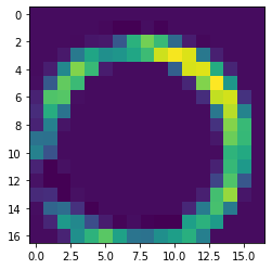
시각화 함수 구현
from lime import lime_image
from lime.wrappers.scikit_image import SegmentationAlgorithm

def display_gradcam_with_img(img,heatmap,alpha=0.4):
  # 0과 1 사이 값을 갖는 행렬 -> 0과 255 사이의 정수를 갖는 행렬로 변환
  heatmap=np.uint8(255*heatmap)

  # 칼라맵 설정
  jet=cm.get_cmap('jet')
  jet_colors=jet(np.arange(256))[:,:3]

  # 0~255에 대응하는 RGB값 불러오기 [256,3]
  jet_heatmap=jet_colors[heatmap] # RGB 이미지가 됨

  # 행렬을 이미지로 바꿔주기
  jet_heatmap=keras.preprocessing.image.array_to_img(jet_heatmap)

  # 히트맵 사이즈를 이미지 크기로 바꾸기
  jet_heatmap=jet_heatmap.resize((img.shape[1],img.shape[0]))

  # 이미지를 행렬로 바꾸기
  jet_heatmap=keras.preprocessing.image.img_to_array(jet_heatmap)

  # 히트맵과 이미지 겹치기
  superimposed_img=jet_heatmap*alpha+img

  superimposed_img=np.uint8(superimposed_img)

  # Saliency 이미지
  sample_saliency_xai_image = vanilla_saliency(model, img / 255) # grad-cam에서 255 곱해줘서 다시 나눠줌
  sample_ig_xai_image = ig(model, img / 255)                     # grad-cam에서 255 곱해줘서 다시 나눠줌


  # 이미지를 슈퍼픽셀로 분할하는 알고리즘 설정
  # quickshift, slic, felzenswalb 등이 존재
  # X_test, y_test = next(iter(test_generator))
  explainer = lime_image.LimeImageExplainer()
  segmenter = SegmentationAlgorithm('slic',
                                    n_segments=100, # 이미지 분할 조각 개수
                                    compactnes=1, # 유사한 파트를 합치는 함수
                                    sigma=1) # 스무딩 역할: 0과 1사이의 float
  exp = explainer.explain_instance(img / 255,
                                  classifier_fn=model.predict, # 40개 class 확률 반환
                                  top_labels=3, # 확률 기준 1~5위
                                  num_samples=100, # sample space
                                  segmentation_fn=segmenter) # 분할 알고리즘
  # 모든 세그먼트 출력
  temp, mask = exp.get_image_and_mask(np.argmax(label),
                                  positive_only=False, # 설명 모델이 결과값을 가장 잘 설명하는 이미지 영역만 출력
                                  num_features=8, # 분할 영역의 크기
                                  hide_rest=False) # 이미지를 분류하는 데 도움이 되는 서브모듈 외의 모듈도 출력

  return img,temp,superimposed_img,sample_saliency_xai_image,sample_ig_xai_image
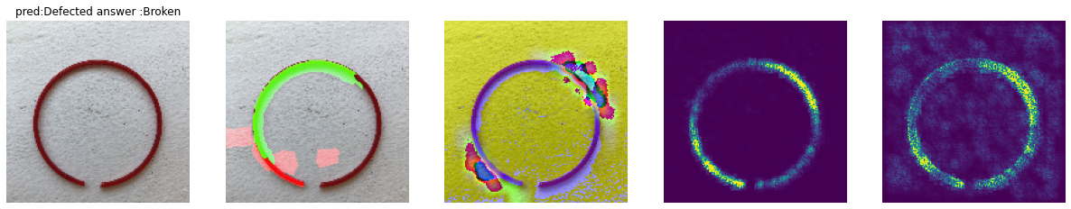
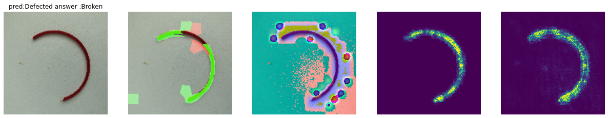
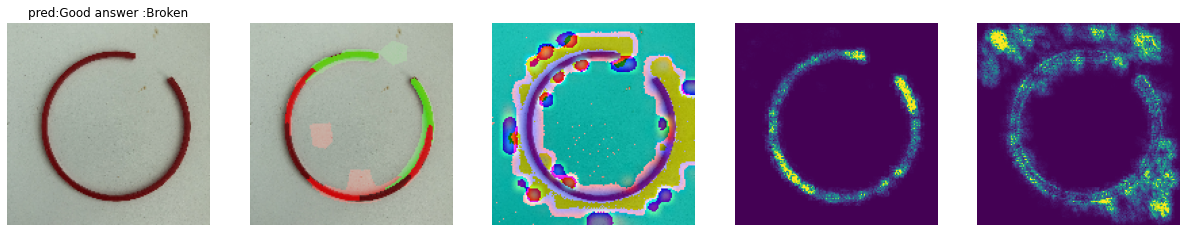
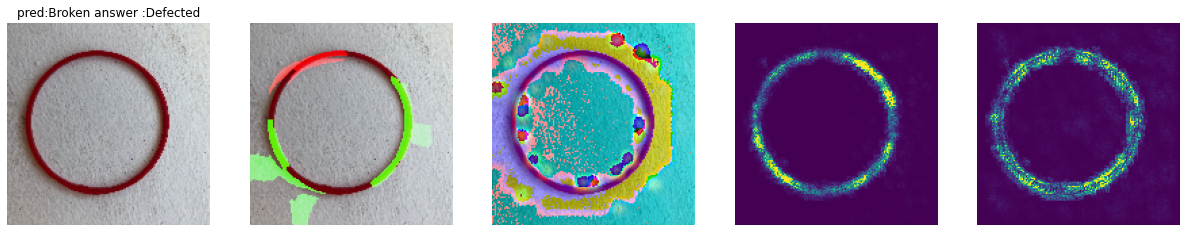
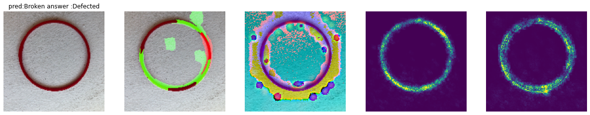
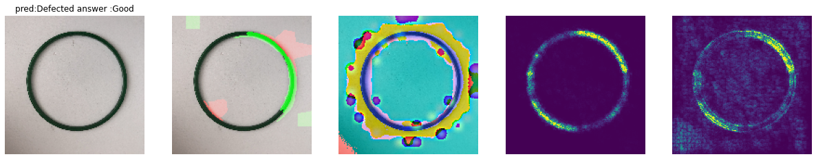
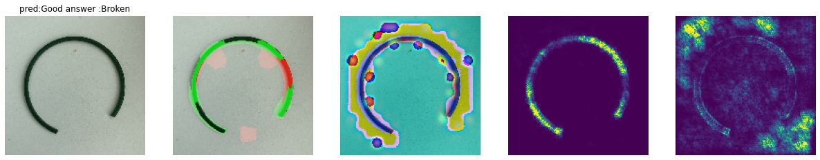
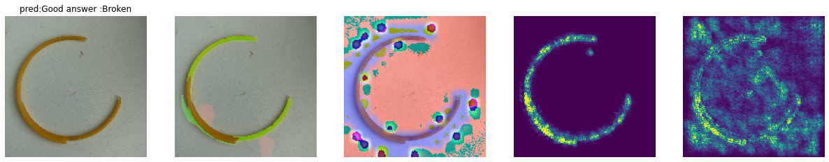
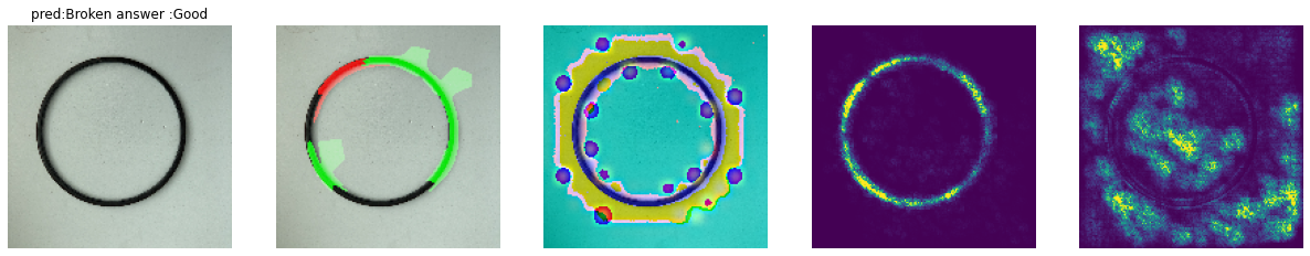
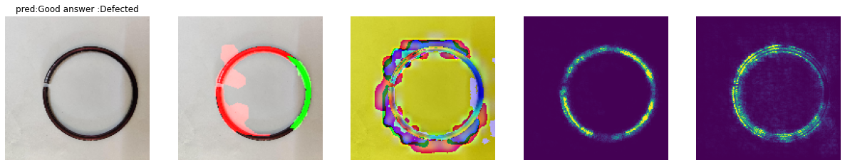
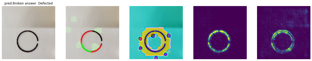
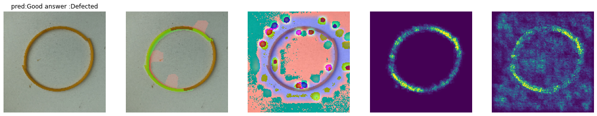
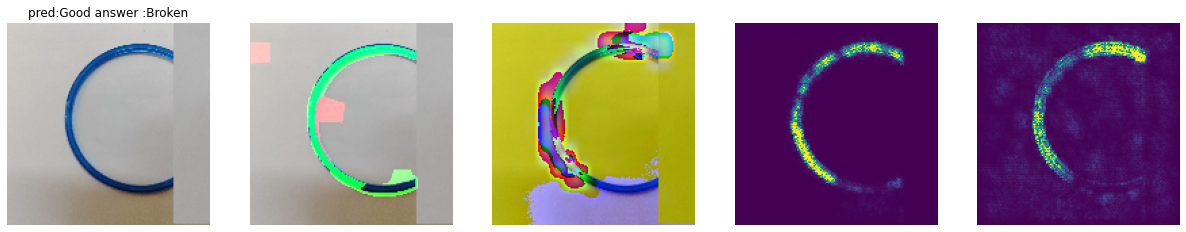
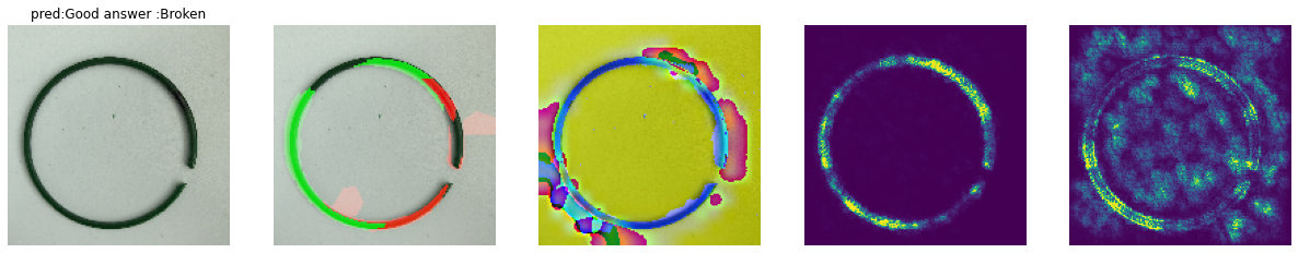
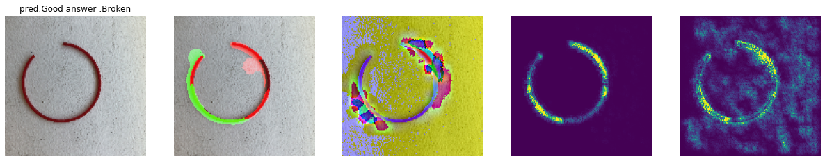
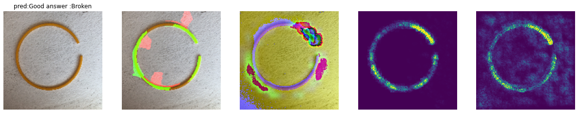
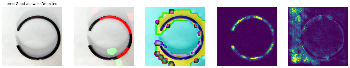
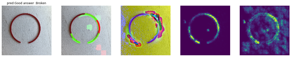
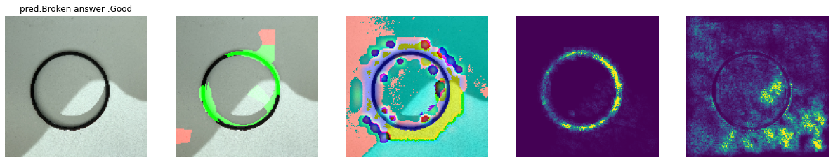
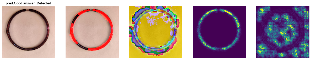
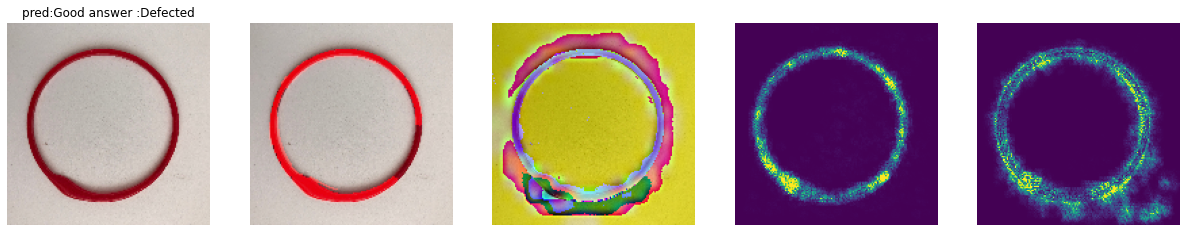
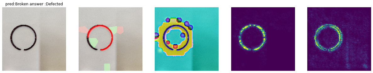
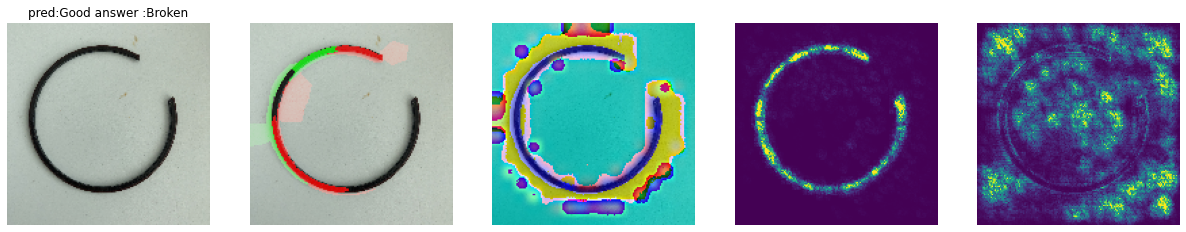
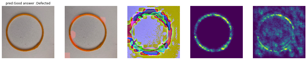
시각화 함수 실행
plt.figure(figsize=(15, 15), dpi=100)
# 반복문을 통해 이미지를 추가해 전체 보이기
for i, (img, label) in enumerate(zip(incorrect_images, incorrect_labels)):
heatmap=grad_cam(img[np.newaxis],model,'max_pooling2d_2')
original_img,temp,superimposed_img,sample_saliency_xai_image,sample_ig_xai_image = display_gradcam_with_img(img*255,heatmap,alpha=0.8)
# 정답 라벨
if correct_labels[i][0]==1:
ans='Broken'
elif correct_labels[i][1]==1:
ans='Defected'
elif correct_labels[i][2]==1:
ans='Good'
# 예측 라벨
if label[0]==1:
pred='Broken'
elif label[1]==1:
pred='Defected'
elif label[2]==1:
pred='Good'
# 시각화
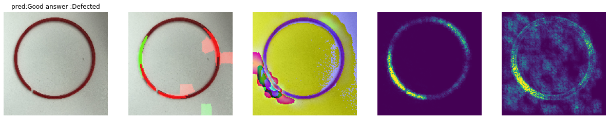
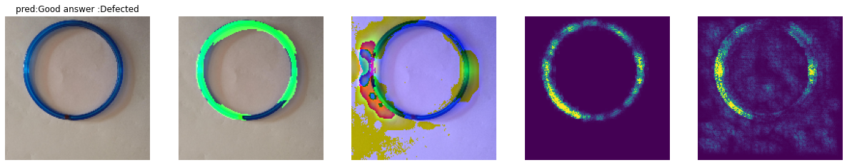
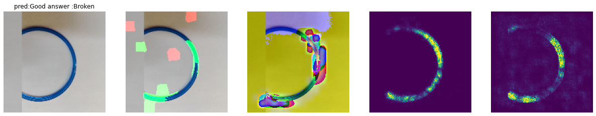
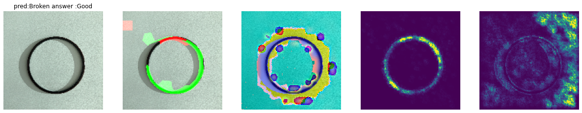
fig, axes=plt.subplots(1,5,figsize=(21,7))
axes[0].imshow(img) # 원본 이미지
axes[1].imshow(temp) #히트맵
axes[2].imshow(superimposed_img) # 원본 + 히트맵
axes[3].imshow(sample_saliency_xai_image)
axes[4].imshow(sample_ig_xai_image)
axes[0].set_title(f'pred:{pred} answer :{ans}')
for ax in axes:
ax.axis('off') #축 눈금이랑 숫자 없애기<ipython-input-51-689a5dd33b6a>:24: RuntimeWarning: More than 20 figures have been opened. Figures created through the pyplot interface (`matplotlib.pyplot.figure`) are retained until explicitly closed and may consume too much memory. (To control this warning, see the rcParam `figure.max_open_warning`).
fig, axes=plt.subplots(1,5,figsize=(21,7))
<Figure size 1500x1500 with 0 Axes>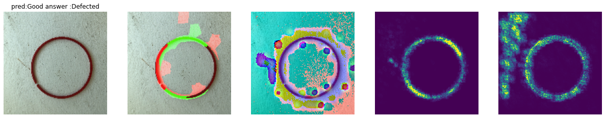


THEO's velog