최종 프로젝트 2주차 day5
2주차 5일째 우린 신규 회원을 유치해야 한다는 분석을 내리고 그에 관련해서 신규 고객 분류를 위한 클러스터링 분석을 하게 되었다.
의미 있는 고객 군집을 찾고 군집 별 역션 플랜을 짜는 것이 오늘의 목표였다.
고객은 2023년 구매를 한 신규 회원을 타겟으로 잡았습니다.
- 고객 별 신규 테이블을 생성
- 고객당 군집을 분류하기 위해 고객 1명에 대한 데이터로 정리
- customer_id
- first_order
- last_orderh
- created_month
- total_order_cnt
- total_price
- purchase_cycle
- total_category_cnt
- order_product_cnt
- avg_order_unit_price
- return_cnt
- return_category_cnt
- avg_order_quantity
- create_to_first_order
- first_month(이후 생성)
- last_month(이후 생성)
=> 16개의 컬럼만을 이용하여 테이블을 만들어서 클러스터링을 해보기로 했다.
- 컬럼별 데이터 분포 현황 확인
#log_scale 변환
pca_sample['total_order_count'] = np.log1p(pca_sample['total_order_count'])
pca_sample['total_price'] = np.log1p(pca_sample['total_price'])
pca_sample['category_count'] = np.log1p(pca_sample['category_count'])
pca_sample['product_count'] = np.log1p(pca_sample['product_count'])
pca_sample['avg_unit_price'] = np.log1p(pca_sample['avg_unit_price'])
pca_sample['return_count'] = np.log1p(pca_sample['return_count'])
pca_sample['avg_purchase_cycle'] = np.log1p(pca_sample['avg_purchase_cycle'])
pca_sample['return_category_count'] = np.log1p(pca_sample['return_category_count'])
pca_sample['create_to_first_order'] = np.log1p(pca_sample['create_to_first_order'])-
클러스터링 할 컬럼 지정
연속형 변수 :
feature_names = ['first_order_month', 'last_order_month', 'create_month', 'total_order_count', 'total_price', 'category_count', 'product_count','avg_unit_price', 'return_count',
'avg_quantity','avg_purchase_cycle','return_category_count','create_to_first_order'] -
데이터 표준화 -> 연속형 (StandardScaler)
-
PCA 갯수 -> 2
-
K-means
-
시각화 ( scatterplot, line )
-
실루엣 계수
를 알아보기로 했다.
코드는 총 3가지를 공유 받았다.
- 클러스터링용 코드 & 고객별 테이블용 코드를 취합했다.
#라이브러리
import pandas as pd
import numpy as np
import matplotlib.pyplot as plt
import seaborn as sns
import datetime as dt
from datetime import timedelta
import matplotlib.pyplot as plt
plt.rc('font', family='NanumBarunGothic')

# ML 알고리즘
from sklearn.preprocessing import StandardScaler
from sklearn.cluster import KMeans
from sklearn.metrics import silhouette_samples, silhouette_score
from sklearn.decomposition import PCA
from sklearn.manifold import TSNE
from sklearn.preprocessing import LabelEncoder
from sklearn.preprocessing import OneHotEncoder
from yellowbrick.cluster import KElbowVisualizer

# 경고 무시
import warnings
warnings.filterwarnings('ignore')

#2023년 신규 가입자
main_order['order_date'] = pd.to_datetime(main_order['order_date'])
main_order['created_at'] = pd.to_datetime(main_order['created_at'])
main_order['created_year'] = main_order['created_at'].dt.year
new_2023 = main_order.query('created_year == 2023')

#고객별 테이블 생성
customer_clustering = new_2023.copy()
customer_clustering['return_status'] = customer_clustering['return_status'].fillna(0)
customer_clustering['return_status'] = np.where(customer_clustering['return_status'] == 0,0,1)
customer_clustering['order_date'] = customer_clustering['order_date']
customer_clustering = customer_clustering.groupby('customer_id').agg(first_order=('order_date','min'),\
                                                                      last_order=('order_date','max'),\
                                                                      created_at=('created_at','min'),\
                                                                      total_order_count=('order_id','count'),\
                                                                      total_price=('total_price','sum'),\
                                                                      category_count=('category','nunique'),\
                                                                      product_count=('product_name','nunique'),\
                                                                      avg_unit_price=('unit_price','mean'),\
                                                                      return_count = ('return_status','sum'),\
                                                                      avg_quantity = ('quantity','mean')).reset_index()


#구매 주기 파악
order_frequency = new_2023[['customer_id','order_date']].sort_values(['customer_id','order_date'],ascending=[True,True])
order_frequency['before_order'] = order_frequency.sort_values('order_date',ascending=True).groupby('customer_id')['order_date'].shift(1)
order_frequency['frequency'] = (order_frequency['order_date'] - order_frequency['before_order']).dt.days
order_frequency = order_frequency.groupby('customer_id')['frequency'].mean().round(0).reset_index().rename(columns={'frequency':'avg_purchase_cycle'})

#테이블 병합
customer_clustering = pd.merge(customer_clustering,order_frequency,on='customer_id',how='left')
customer_clustering = pd.merge(customer_clustering,new_2023[new_2023['return_status'].isna() == False].groupby('customer_id')['category'].nunique().reset_index().rename(columns={'category':'return_category_count'}),how='left',on='customer_id')
customer_clustering['return_category_count'] = customer_clustering['return_category_count'].fillna(0)
customer_clustering['create_to_first_order'] = (customer_clustering['first_order'] - customer_clustering['created_at']).dt.days
customer_clustering['avg_purchase_cycle'] = customer_clustering['avg_purchase_cycle'].fillna(0)

customer_clustering

#PCA(주성분 분석) n = 2
pca_main = customer_clustering.copy()

#날짜변수 처리
pca_main['first_order_month'] = pca_main['first_order'].dt.month
pca_main['last_order_month'] = pca_main['last_order'].dt.month
pca_main['create_month'] = pca_main['created_at'].dt.month

#컬럼 선택
feature_names = ['first_order_month', 'last_order_month', 'create_month',
                  'total_order_count', 'total_price', 'category_count',
                  'product_count','avg_unit_price', 'return_count',
                  'avg_quantity', 'avg_purchase_cycle','return_category_count',
                  'create_to_first_order']
pca_sample = pca_main[feature_names]

#log_scale 변환
pca_sample['total_order_count'] = np.log1p(pca_sample['total_order_count'])
pca_sample['total_price'] = np.log1p(pca_sample['total_price'])
pca_sample['category_count'] = np.log1p(pca_sample['category_count'])
pca_sample['product_count'] = np.log1p(pca_sample['product_count'])
pca_sample['avg_unit_price'] = np.log1p(pca_sample['avg_unit_price'])
pca_sample['return_count'] = np.log1p(pca_sample['return_count'])
pca_sample['avg_purchase_cycle'] = np.log1p(pca_sample['avg_purchase_cycle'])
pca_sample['return_category_count'] = np.log1p(pca_sample['return_category_count'])
pca_sample['create_to_first_order'] = np.log1p(pca_sample['create_to_first_order'])

#정규화
scaler = StandardScaler()
pca_sample_scaled = scaler.fit_transform(pca_sample)

#PCA 실행
pca = PCA(n_components=2)
printcipalComponents = pca.fit_transform(pca_sample_scaled)
principal_df = pd.DataFrame(data=printcipalComponents, columns = ['principal component1', 'principal component2'])
principal_df.head(5)

#설명력 체크
print(pca.explained_variance_ratio_)
print(sum(pca.explained_variance_ratio_))

#Elbow Method
model = KMeans()
# k 값의 범위를 조정해 줄 수 있습니다.
visualizer = KElbowVisualizer(model, k=(3,10))
# 데이터 적용
visualizer.fit(principal_df)
visualizer.show()

#클러스터링
optimal_k = 5
kmeans = KMeans(n_clusters=optimal_k, random_state=42, init = 'k-means++')
clusters = kmeans.fit_predict(principal_df)
principal_df['cluster'] = kmeans.labels_

#군집별 라인그래프
pca_sample_cluster = pd.DataFrame(pca_sample_scaled)
pca_sample_cluster.columns = feature_names
pca_sample_cluster
pca_sample_cluster['cluster'] = kmeans.labels_
pca_sample_cluster.groupby('cluster').mean().T.plot(figsize=(15,10))

# kmeans 시각화
plt.figure(figsize=(15, 10))
sns.scatterplot(data=principal_df, x='principal component1', y='principal component2', hue='cluster', palette='viridis')
plt.title('KMeans Clustering Results')
plt.xlabel('PCA 1')
plt.ylabel('PCA 2')
plt.show()


#해당 군집화 실루엣 계수
score_samples = silhouette_score(principal_df, kmeans.labels_)
principal_df['silhouette_coeff'] = score_samples
print(np.mean(score_samples))- 컬럼들을 이것저것 빼보고 클러스터링을 진행해 보았다.
- 그리고 우리는 로그 스케일링을 진행 후 모든 컬럼을 사용하고 K=4로 클러스터링을 진행한 것을 사용하기로 확정했다.
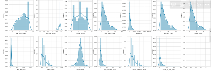
🔼로그 스케일링 (전) 컬럼 분포
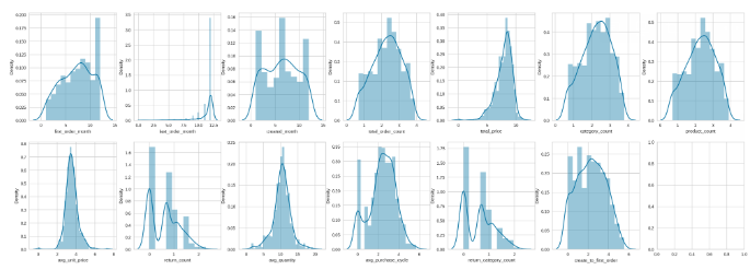
🔼로그 스케일링 (후) 컬럼 분포 → 일부 컬럼에서 나타났던 왜도 문제 보완
클러스터링 결과에 대한 신뢰도를 높이고자
[클러스터링 과정 요약]
- 선정한 컬럼(파생 변수에 대한 설명 포함 -> 계산식 같은)
->왜 우리가 이런 테이블을 구성하게 되었는가에 대한 내용 언급 - 로그화 및 정규화 진행 이유
컬럼 분포 확인 결과 정규분포를 따르지 않는 컬럼확인(이전)
로그 스케일링을 통해 정규화를 진행하여 일부 컬럼에서 나타난 왜도 문제 보완(후)
컬럼 간 범위 차이를 줄여주기 위해 정규화 진행하여 클러스터링 결과 도출
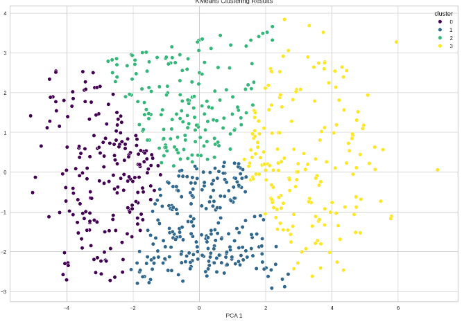
2023년도 신규 고객만 해당하는 라인그래프
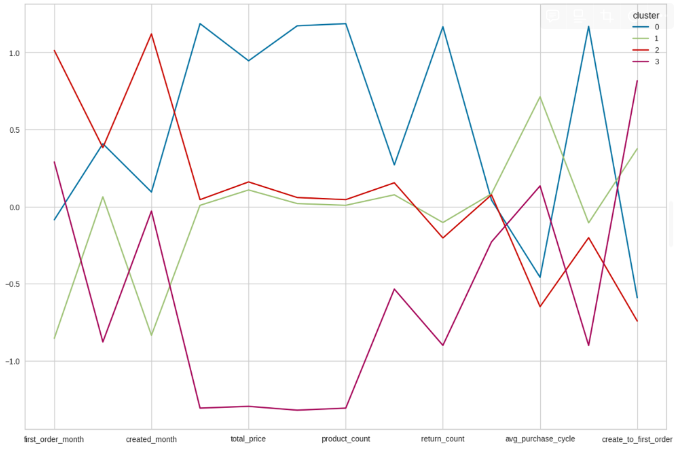
🔼클러스터링 결과 및 클러스터별 라인 그래프
해당 클러스터링 분산 설명력: 0.6 , 실루엣 계수: 0.43
- 0번 클러스터 (파란색)
-> 일주일 이내의 짧은 주기로, 평균 이상의 구매 횟수(약27회) 및 약 27종류의 제품 구매, 첫 구매가지 일주일 가량(단기간 구매), 평균적으로 13000달러 매출 발생
-> 카테고리 : 1,2,3위 까지 컴퓨터 관련
=> 전체 주문 건수, 전체 구매 금액,카테고리 수,제품수,평균 객단가,반품 수,반품 카테고리 수가 제일 높게 나옴
=> 아이디를 만들고 첫주문부터 마지막 주문까지 구매주기가 긴것을 볼 수 있음. 하지만 전체적으로 주문 건수나 주문하는 제품의 수, 구매 금액, 객단가가 높은 것을 볼수 있고, 그것에 비례하여 반품하는 카테고리와 제품의 수가 높은것을 알수 있다. 구매 주기는 낮은 것으로 보인다.
=> 0번 클러스터에 포함되어 있는 고객들의 데이터를 확인햇을땐 구매 주기가 일주일 단위로 짧다고 한다. 그러면 기준선 아래도 내려가면 구매 주기가 짧다고 생각하면 될까?
=> 1년 내내 다양한 상품을 많이 자주 구매하는 사람들
=> 충동 구매자
=> 제발.. 해석 좀... 되라..... 굳이 낮은걸 해석할 필요는 없나?
- 1번 클러스터 (녹색)
-> 한 달 가량의 보통 주기로 구매, 평균적인 구매 횟수 (약 10회) 및 10종류의 제품 구매, 첫 구매까지 4주 가량 소모, 평균적으로 4400달러 매출 발생
-> 카테고리 : 5위 안에 컴퓨터
=> 구매주기가 제일 긴 것으로 확인되는 그래프이다.
- 2번 클러스터 (빨간색)
-> 일주일 이내의 짧은 주기로 구매, 평균적인 구매 횔수 (약10회) 및 10종류의 제품 구매, 첫 구매까지 5일정도 소모 (단기간 구매), 평균적으로 3400달러 매출 발생
-> 카테고리 : 5위 안에 컴퓨터
=> 아이디를 생성하고 첫 주문하는 달이 높은 값을 보임.
=> 구매 주기가 제일 아래로 가있기 때문에 제일 짧은 구매 주기를 보인다.
- 3번 클러스터 (자주색)
-> 한 달 가량의 보통 주기로 구매, 구매 횟수와 제품의 종류가 적음(2회,2종류), 평균적으로 800달러의 매출 발생, 첫 구매까지 약 2달정도 소모 (너무 길음)
-> 카테고리 : 1. 진공청소기 2. TV 3.여성시계 8. 컴퓨터
<기준선을 기준으로 컬럼들 해석 >
=> total_price,total_order_count, category_count, product_count, avg_unit_price → 기준선에서 높으면 긍적적인 방향으로 높은 수치라고 보면 된다.
=> return_count → 높으면 높을수록 반품 수량이 많다.
=> avg_purchase_cycle → 기준선보다 낮으면 구매 주기가 짧다고 생각하면 된다.
=> 클러스터링을 해석할 때 분석가들의 해석이 중요하다는 생각이 들었다.
어제부터 해석을 해보려고 봤지만.. 어떻게 해석을 해야할지 고민이 된다.
gpt친구에게도 물어보고 비교해보지만 왜 저런 다른 해석이 나오는지 모르겠다.
=> 기준인 0.0보다 낮으면 어떤 컬럼에서는 좋은게 되고 어떤 컬럼에서는 반대로 해석이 되는 것이 어떤 기준을 잡고 해석을 해야하는것일까? 무슨 기준일까??? ...넌 기준이 무엇이니.....
회사의 문제점과 개선점을 찾았을 때
신규 고객 유치에 미온적인 태도를 취하고 있음을 유추할 수 있었다.
이에 따라 신규 고객 유치의 중요성과 현황을 알기 위해
신규 고객들의 현황과 이들의 구매 경향, 매출에 미치는 영향을 확인하였다.
이 후, 신규 회원 유치 방안에 대하여 분석을 해보고자 하였으나,
마케팅 데이터 및 고객 세부 데이터가 부재하였고
현재 제공 받은 데이터를 토대로
최근 1년내 주문을 했던 신규 고객들은 어떤 구매경향을 가지고 있는지
고객 분류를 해보기 위해 클러스터 분석을 해보았다.
⇒ 2023년 신규 구매자들의 구매경향은 위와 같이 총 4가지의 분류로 나뉘었다.
이 중 가장 많은 매출을 발생한 고객군집은 0번으로 ,
이들은 다양한 제품들을 구매하고, 짧은 기간 내에 재구매 횟수가 높은 구매 성향을 지녔다.
또한 그 중 컴퓨터 관련 제품군이 가장 매출이 높았으며, 다양한 제품들을 구매하였기 때문에 큰 차이는 없었으나 그 중 가장 많이 찾았던 제품은 ~~이다..
이런 구매 성향을 지닌 고객군들의 매출을 더욱 높이기 위해
다양한 제품군을 유치하고 구매 횟수에 따른 로열티(리워드 프로그램) 등을 제공하는 등의 마케팅 전략과 매출이 가장 높았던 컴퓨터 관련 제품군에 대한 가격 최적화를 진행 해보는 방안을 제안한다.
또한 해당 고객군들은 반품 서비스 이용률 이 높기 때문에
반품절차 간소화에 관한 마케팅을 시도해 보는 것도 방법이 될 수 있다.
=> 클러스터링을 좀더 생각해보고 아래 결론부분도 다시 한번 생각해보려고 한다.
하지만, 지금 위에 적혀있는 결론은 팀원들과 이야기하고 나온 결론과 결과라고 생각하면 된다.