<인공신경망> 11. 고속 optimizer와 regularization

📌 Faster Optimizers

1. Speed up training

🔸 Good initialization strategy for the connection weights => 적절한 parameter 초기화 방법
🔸 Good activation function
🔸 Batch normalization => network의 입력과 출력의 분포 정규화
🔸 reusing parts of a pretrained network

2. Faster optimizer than regular Gradient Descent optimizer

🔸 optimizer도 학습 속도를 높이는데 도움이 됨
🔸 원래는 Gradient Descent optimizer인 SGD를 주로 사용했는데 이보다 더 좋은 optimizer 존재할 경우 사용

1) Momentum optimization, NAG(Nesterov Accelerated Gradient), AdaGrad, RMSProp, and finally Adam(+Adamax, Nadam) optimization

2) Almost always use Adam optimization

optimizers.SGD -> optimizers.Adam

3) Application of optimizers: dataset dependent

💡 대부분 Adam optimizer 사용해서 성능이 좋아지는데 그렇지 않을 경우, Adam, Adam variants, RMSProp 순서로 진행해보고 그래도 성능이 좋아지지 않을 경우 Nesterov, Pure momentum 순서로 진행 => Pure momentum의 경우 성능이 나빠지는 경우가 거의 없음. 이 순서 암기
🔸 Adaptive optimization (Adam, Adam variants, RMSProp)
🔸 Nesterov
🔸 Pure momentum

📌 Optimizer comparison

*: bad, **: average, ***:good

class	convergence speed:학습속도	convergence quality:학습결과	특징
SGD	*	***	.
SGD(momentum=0.9)	**	***	pure momentum optimizer 사용
SGD(momentum=0.9, nesterov=True)	**	***	NAG optimizer 사용
Adagrad(lr=)	***	*(stops too early)	.
RMSprop(lr=..., rho=0.9)	***	** or ***	rho argument는 0.9가 default. 거의 바꾸지 X
Adam(lr=..., beta_1=0.9, beta_2=0.999)	***	** or ***	beta_1, beta_2는 해당 수가 default. 거의 바꾸지 X
Nadam(lr=..., beta_1=0.9, beta_2=0.999)	***	or *	'''
AdaMax(lr=..., beta_1=0.9, beta_2=0.999)	***	or *	'''

🔸 Pure momentum과 NAG optimizer는 SGD 기반의 optimizer로 SGD의 argument 설정에 따라 optimizer 달라짐
🔸 Adagrd, RMSprop, Adam, Nadam, AdaMax는 keras의 optimizer library에 내장되어있음. 대부분 learning rate만 결정해주면 됨 (rho, beta_1, beta_2는 거의 바꾸지 않고 default 사용)
🔸 학습 결과가 중요한 경우 SGD를 사용하고 학습 속도가 중요한 경우는 Adagrad부터 Adamax까지의 optimizer 사용 => But 학습 결과는 데이터에 따라 다름

📌 Learning Rate Scheduling

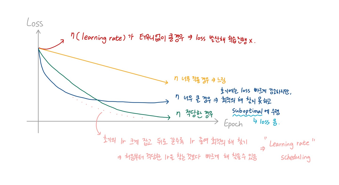
1. Start with a high learning rate => reduce it once it stops making fast progress

🔸 learning rate를 크게 잡아서 loss가 빠르게 떨어지다가 떨어지는 속도가 완만해지면 learning rate 줄임 => optimal constant learning rate보다 optimal solution을 빠르게 찾을 수 있음
🔸 faster than with the optimal constant learning rate

🔸 "몇 epoch이 지났을 때 learning rate를 얼마나 떨어트릴 것인지" : Scheduling

2. Power scheduling

🔸 $η(t)$ = $η_{0}$$(1+t/s)^-c$. hyperparameter c=1 typically, s: steps. t: iteration number
=> c는 주로 1이므로 결국 $η(t)$ = $η_{0} \over 1+t/s$
🔸 t가 증가할 때마다 분모가 커지므로 learning rate는 지속적으로 감소하고, s 값에 따라 감소하는 정도가 달라짐
🔸 Similar to exponential scheduling, but the learning rate drops much more slowly

iteration
한 번의 epoch은 데이터 세트를 전부 사용하여 학습하는 과정이고 한 번의 iteration을 할 때마다 정해진 batch size의 데이터 사용
Ex. dataset이 1000개이고 batch size가 100이라면, 한 번의 epoch은 10개의 iteration으로 구성. 각 iteration에서는 모델이 100개의 데이터를 처리

3. Exponential scheduling

🔸 $η(t)$ = $η_{0}$ $10^-t/s$
🔹 step에 해당하는 s 값에 따라 감소하는 속도를 조절할 수 있음
🔸 Requires tuning $η0$ and s => tuning해야할 hyperparameter
🔸 The learning rate will drop by a factor of 10 every s steps
🔹 s step마다 learning rate 1/10로 감소

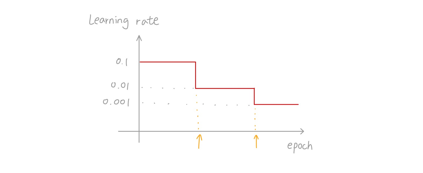
4. Piecewise constant learning rate

🔸 일정한 epoch동안 일정한 learning rate(0.1 -> 0.01 -> 0.001)를 가짐
🔸 Constant learning rate for a number of epochs, and step down it (0.1 -> 0.01 -> 0.001)
🔸 Finding the right learning rates and the duration => 특정 learning rate로 유지되는 epoch의 수와 learning rate 값을 정하는 것이 관건

5. Performance scheduling

🔸 Measure the validation error every N steps (just like for early stopping) => reduce the learning rate by a factor of when the error stops dropping
🔹 validation error를 기준으로 해서 validation error가 줄어들지 않으면 learning rate 감소

6. 1 cycle scheduling

1. Linearly $η_{0}$->$η_{1}$ halfway through training
2. $η_{1}$->$η_{0}$(떨어지는 방향) again durin the second half of training
3. finishing the last few epochs by dropping the rate down by several orders of magnitude (linearly)
   🔸 => train 기간의 절반동안 $η_{0}$에서 $η_{1}$로 linear하게 증가 -> 나머지 기간동안 $η_{1}$에서 $η_{0}$로 감소 -> 마지막 몇 epoch에서 급격하게 lr를 줄여 학습 진행
   
   
   🔸 $η_{1}$: optimal learning rate. $η_{0}$은 $η_{1}$의 1/10배(=10배 작은 값)
   🔸 Momentum: high(0.95) -> low(0.85) => high linearly, keeping high for the last few epochs
   🔹 learning rate와 함께 momentum도 함께 변화시킴
   

7. Code

1) power scheduling: decay=1/s, c=1

optimizer = keras.optimizers.SGD(lr=0.01, decay=1e-4)

🔸 decay가 1/10000이므로 step s=10000
🔸 lr이 초기 learning rate $η_{0}$에 해당하는 값

2) LearningRateScheduler callback: update the optimizer's learning_rate attribute at the beginning of each epoch

🔸 각 epoch이 시작할 때 optimizer의 learning_rate attribute를 exponential_decay함수에 따라 업데이트

def exponential_decay(lr0, s):
	def exponential_decay_fn(epoch):
    	return lr0 * 0.1 **(epoch/s)
    return exponential_decay_fn
exponential_decay_fn = exponential_decay(lr0=0.01, s=20)
lr_scheduler = keras.callbacks.LearningRateScheduler(exponential_decay_fn)
history = model.fit(X_train_scaled, y_train, [...], callbacks=[lr_scheduler])

3) Exponential scheduling: epoch starts with 0

🔸 current learning rate를 함수의 second parameter로 가지는 경우, 현재 lr의 원하는 연산을 해 해당 lr로 줄일 수 있음

def exponential_decay_fn(epoch, lr)
	return lr*0.1**(1/20)

4) piecewise constant scheduling

def piecewise_constant_fn(epoch):
	if epoch<5:
    	return 0.01
    elif epoch<15:
    	return 0.005
    else:
    	return 0.001

5) Performance scheduling: ReduceLROnPlateau callback

lr_scheduler = keras.callbacks.ReduceLROnPlateau(factor=0.5, patience=5)

🔸 0.5 x lr whenever the validation loss does not improve for five epochs => 5 epoch동안(patience) 변화가 없으면 lr을 0.5(factor)로 변화(lr이 절반으로 감소)

6) Keras: use keras.optimizers.schedules => updates the learning rate at each step

🔸 함수를 별도로 정하지 않고도 각 step마다 learning rate를 업데이트시킬 수 있음
🔸 아래 코드에서는 learning rate가 초기값 0.01에서 매 step마다 0.01x$0.1^s$ 로 변화
🔸 specific to tf.keras => tensorflow의 keras에만 있으므로 tensorflow를 사용하지 않을 경우 사용할 수 없음

s = 20*len(X_train) // 32
learning_rate = keras.optimizers.schedules.ExponentialDecay(0.01, s, 0.1)
optimizer = keras.optimizers.SGD(learning_rate)

📌 Avoiding Overfitting Through Regularization

1. DNN: typically tens of thousands of parameters, sometimes even millions

1) incredible amount of freedom and can fit a huge variety of complex datasets

🔸 DNN이 수천개 이상의 parameter를 가지고 있다는 것은 자유도가 높아 복잡한 모델을 만드는데 사용할 수 있고 복잡한 데이터셋을 학습시킬 수 있다는 것을 의미 => dataset의 instance가 충분하지 않거나 종류가 다양하지 않을 경우 overfitting의 가능성도 크다는 것 의미

2) prone to overfitting => regularization is necessary

3) Ex. Early Stopping (ch.10)

2. $l_{1}$ and $l_{2}$ Regularization (ch.4)

🔸 l1_l2는 L1L2와 거의 동일
🔸 l1은 sparse model(=> weight가 0에 가까운 값들이 많고 0이 아닌 의미있는 값을 가지는 weight가 거의 없는 모델)의 경우 주로 사용, 그렇지 않을 경우 l2 사용
🔸 코드에 사용할 때 kernel_regularizer argument에 원하는 regularization assign해 사용
🔸 학습을 진행하는 중 overfitting이 발생하면 regularization 설정해 학습해보기. 그래도 안 좋다면 다른 방식의 regularization 사용

1) 각 Dense layer마다 activation, initialization, regularization 진행

l1 = tf.keras.regularizers.l1(l=0.01)
l2 = tf.keras.regularizers.l2(l=0.01)
l1_l2 = tf.keras.regularizers.l1_l2(l1=0.01, l2=0.01)
L1L2 = tf.keras.regularizers.L1L2(l1=0.01, l2=0.01)

model7 = keras.Sequential([
	# 앞에 정의한 후 사용
	keras.layers.Dense(n_hidden1, kernel_initializer=he_init, kernel_regularizer=l1, activation=leaky_relu),
    keras.layers.Dense(n_hidden2, kernel_initializer=he_init, kernel_regularizer=l2, activation=leaky_relu),
    # 바로 정의해 사용
    keras.layers.Dense(n_hidden3, kernel_initializer=he_init, kernel_regularizer=tf.keras.regularizers.li(l=0.02), activation=leaky_relu),
    keras.layers.Dense(n_hidden2, kernel_initializer=he_init, kernel_regularizer=l1_l2, activation=leaky_relu),
    keras.layers.Dense(n_hidden2, kernel_initializer=he_init, kernel_regularizer=L1L2, activation='softmax'),
])

2) 같은 activation, initialization, regularization 사용할 경우

🔸 object 생성 후 지정되지 않은 값 넣어서 사용
🔸 변경하고 싶을 경우 사용할 때 해당 argument 새로 지정

from functools import partial
RegularizedDense = partial(keras.layers.Dense, activation="elu", kernel_initializer="he_normal", kernel_regularizer=keras.regularizers.l2(0.01))

model = keras.models.Sequential([
	keras.layers.Flatten(input_shape=[28,28]),
    RegularizedDense(300),
    RegularizedDense(100),
    RegularizedDense(10, activation="softmax", kernel_initializer="glorot_uniform")
])

3. Dropout (Hinton, 2012)

1) The most popular regularization techniques: 1-2% accuracy boost

🔸 regularization 뿐만 아니라 accuracy 향상에도 도움

2) Every neuron is entirely ignored during a training step with a probability p

🔸 => training step동안 p라는 확률로 neuron 무시하고 학습 진행. 특정한 neuron이 무시될 확률은 p.
🔸 => output layer에서는 dropout하지않고, input layer와 hidden layer에 대해서만 dropout 가능
🔸 Applied temporarily in a step; determined again in the next step
🔹 각 step마다 특정 neuron을 무시할지말지 결정. 다음 step에서는 동일한 확률을 가지고 neuron 무시할지말지 결정
🔸 Hyperparameter p=0.1~0.5 typically. 0.2~0.3 in RNN, 0.4~0.5 in CNN
🔸 Dropout is not applied for inferencing => dropout은 train할 때에만 적용하며 inference(=test)할 때에는 적용하지 않음
🔸 아래 그림은 p=0.5

3) DNN with dropout

🔸 Less sensitive to slight changes in the inputs, more robust network that generalizes better => input에서의 작은 변화에 덜 예민하며 새로운 데이터를 넣었을 때 (generalize했을때) 더 성능이 좋음
🔹 특정한 neuron의 weight가 커서 미치는 영향이 컸을 경우 그 neuron에 대해 학습을 많이 진행하는데, 이가 dropout되었을 때에는 다른 다양한 neuron에서도 학습을 많이 진행할 수 있어 generalize했을 때 성능이 더 좋게 나타남
🔸 Averaging ensemble of different neural networks (sharing weights) => step1과 step2의 network 모양은 같지 않지만 network의 weight는 같아 ensemble average 형태로 학습을 진행하는 것과 같아 성능이 좋아짐

ensemble average
하나하나의 estimate 성능은 좋지 않더라도 ensemble learning하게 되면 훨씬 좋은 성능의 결과를 얻을 수 있음

4) Inferencing

🔸 All neurons are connected => output is increased by 1/(1-p)
🔹 inference시에는 dropout이 일어나지 않으며, output은 train했을 때와 비교했을 때 1/(1-p)만큼 큼 => input이 6개이고 dropout의 p가 1/3이라했을 경우, train 시의 output은 4개의 neuron을 더한 값이고 test(inference)의 output은 6개의 neuron을 더한 값이기 때문에 inference의 output이 크게 나타남 => 따라서 compensation(보상) 필요
🔸 Compensation: multiply each input connection weight by (1-p) after training
🔹 => inference 시 (1-p)를 곱해 output 값 줄임. (1-p는 1보다 작은 값)
🔸 Alternatively, divide each neuron's output by (1-p) during training
🔹 => train 시 (1-p)로 나눠 output 값 증가
🔹 It is not perfectly equivalent, but they work equally well: 둘 다 output을 완전히 일치시키는 것은 아니지만 잘 동작함

5) Code

🔸 dropout은 각 hidden layer의 입력 쪽에서 작용
🔸 dropout을 하면 그 뒤에 나오는 layer에 영향 미침
🔸 dropout을 하면 각 neuron이 학습에 의해 weight가 update되는 횟수가 실제 step 수보다 작을 수밖에 없음

model = keras.models.Sequential([
	keras.layers.Flatten(input_shape=[28,28]),
    keras.layers.Dropout(rate=0.2),	#입력neuron 중 0.2의 확률로 hidden layer에 들어감
    keras.layers.Dense(300, activation="elu", kernel_initializer="he_normal"),
    keras.layers.Dropout(rate=0.2),
    keras.layers.Dense(100, activation="elu", kernel_initializer="he_normal"),
    keras.layers.Dropout(rate=0.2),
    keras.layers.Dense(10, activation="softmax")
])

6) Tend to significantly slow down convergence

🔸 => 학습 속도 느려지지만 inference 속도는 변하지 않음(dropout은 train 시에만 적용)
🔸 However, results in better models if properly used

7) Validation

🔸 overfitting; but similar training and validation losses
🔹 dropout 적용한 train loss와 validation loss는 비슷
🔸 evaluate the training loss without dropout (after training)
🔹 train이 끝난 후 dropout 없이 training loss를 계산했을 때 해당 train loss와 validation loss 비교해 overfitting이 발생했는지 확인

8) Tweaking

🔸 Overfitting: increase the dropout rate
🔹 => regularization 강화
🔸 Underfitting: decrease the dropout rate
🔹 => regularization이 심하게 적용되면 weight값의 변화 범위가 줄어들어 제대로 학습 X underfitting 발생. 따라서 regularization 줄여야함
🔸 increase the dropout rate for large layers, and reduce it for small ones
🔹 layer의 neuron이 많으면 dropout rate를 늘리고, neuron이 적으면 dropout rate 감소
🔸 many state-of-the-art architectures only use dropout after the last hidden layer
🔹 => 요즘은 lower layer보다 high layer에 적용하는 것이 성능이 더 좋아 자주 사용

9) Alpha dropout

🔸 For a self-normalizing network based on the SELU activation function
🔸 Preserves the mean and standard deviation of its inputs
🔹 => self-normalizing network의 경우 입력의 평균과 표준편차를 유지하는 것이 중요
🔸 Regular dropout would break self-normalization
🔹 => regular dropout을 사용할 경우 self-normalization을 파괴하여 regular dropout이 아닌 alpha dropout을 사용해야함

4. Max-Norm Regularization

🔸 weight값이 일정 범위를 벗어나지 못하도록 regularization

1) $||w||_{2} <= r$

🔸 w: incoming weight
🔸 r: max-norm hyperparameter => reducing r increases the amount of regularization => helps to reduce overfitting
🔹 r을 작게 설정하면 regularization 커져 overfitting 줄여줌
🔸 Implementation: $w$<= $wr\over ∣∣w∣∣_{2}$
🔹 ∣∣w∣∣_{2}가 r보다 작으면 그대로 쓰고 크면 위의 식으로 변환

2) Help alleviate the vanishing/exploding gradients problems without Batch normalization

🔸 => BN 사용하면 regularization 사용할 필요 없음

3) Ex.

MaxNorm = tf.keras.constraints.MaxNorm(max_value=1, axis=0)
keras.layers.Dense(n_hidden1, kernel_initializer=he_init, kernel_constraint=MaxNorm, activation="relu")

🔸 CNN: use appropriate axis. usually axis=[0,1,2]
🔸 => 코드상에서 사용하는 데이터가 1D라 axis=0 사용

📌 Summary and Practival Guidelines

1. Default DNN configuration

🔸 momentum optimization은 dataset에 영향을 받지 않아 가장 먼저 사용. Adam 먼저 사용하면 학습 시간 길어짐. momentum 이후 학습 결과가 더 좋은 모델을 찾고싶으면 Adam부터 차례대로 내려가면서 학습
🔸 1 cycle이 아니더라도 계속해서 모니터링 가능하면 원하는대로 customize

2. DNN configuration for a self-normalizing net

🔸 normalization: 이 자체가 self-normalization이기 때문에 별도의 normalization은 필요없지만 input feature에 대한 normalization은 반드시 필요

3. Exception: 예외

🔸 sparse model(weight가 대부분 0)의 경우
=> use l1 regularization and optionally zero out the tiny weights after training: l1 사용하고 train 이후의 작은 weight들은 0으로 만듬
🔸 low-latency model(inference 시 빠른 속도 요구)의 경우
=> (1)fold the Batch Normalization layers into the previous layers, and (2)use a faster activation function such as leaky ReLU or just ReLU, (3)reduce the float precision from 32 bits to 16 or even 8 bits: BN layer를 이전의 layer에 포함시켜 한 번에 계산, 빠른 activation function 사용, double(64bits) precision에서 16 또는 8 bit precision으로 줄여 연산시간 줄임