머신러닝이란
머신러닝
- 명시적으로 프로그래밍하지 않고도 컴퓨터에 학습할 수 있는 능력을 부여하는 학문
- 경험이 쌓여 감에 따라 주어진 태스크의 성능이 점점 좋아질 때 컴퓨터 프로그램은 경험으로 학습한다고 할 수 있음
1. 데이터 관찰
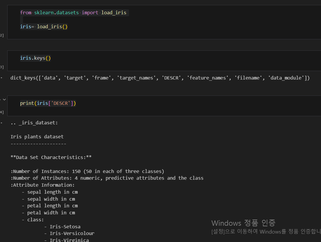
iris 데이터 활용하기
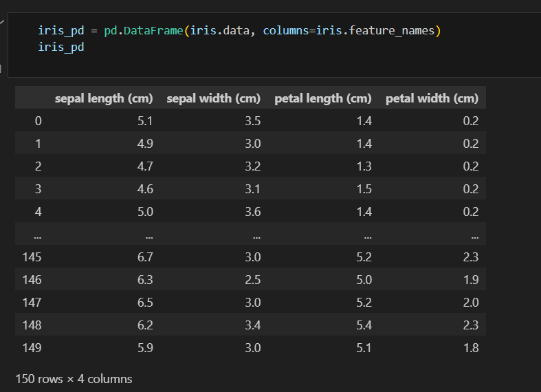
데이터프레임 만들기
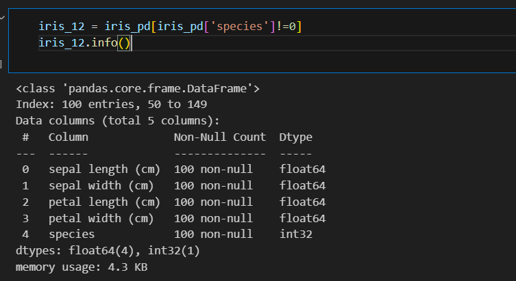
칼럼에 품종 정보 추가하기
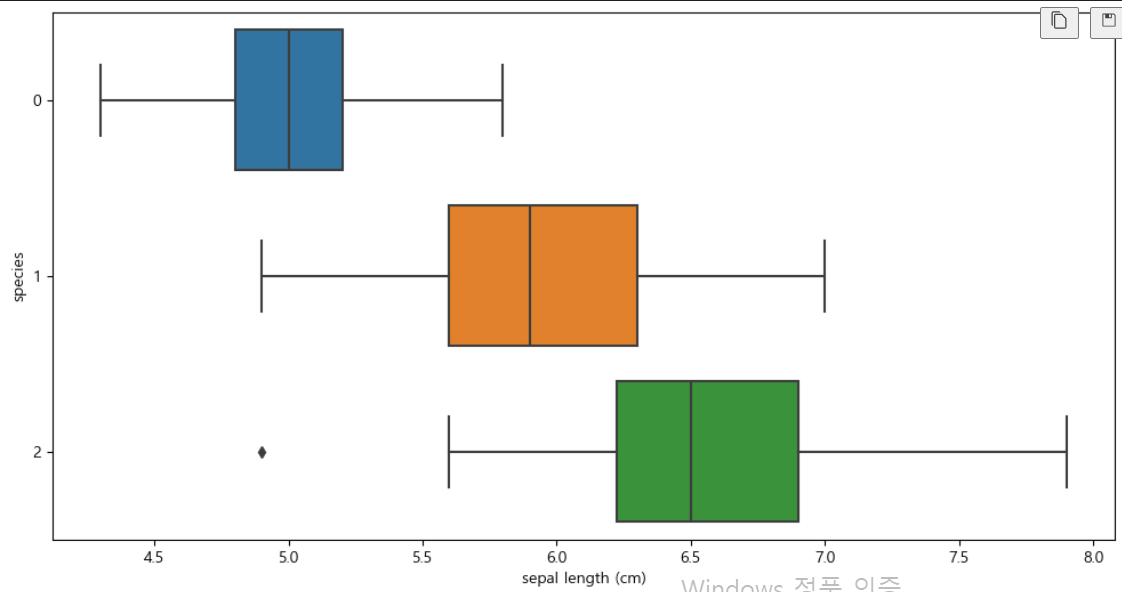
boxplot(x='sepal length (cm)')
plt.figure(figsize=(12,6))
sns.boxplot(x='sepal length (cm)', y='species', data=iris_pd, orient='h')
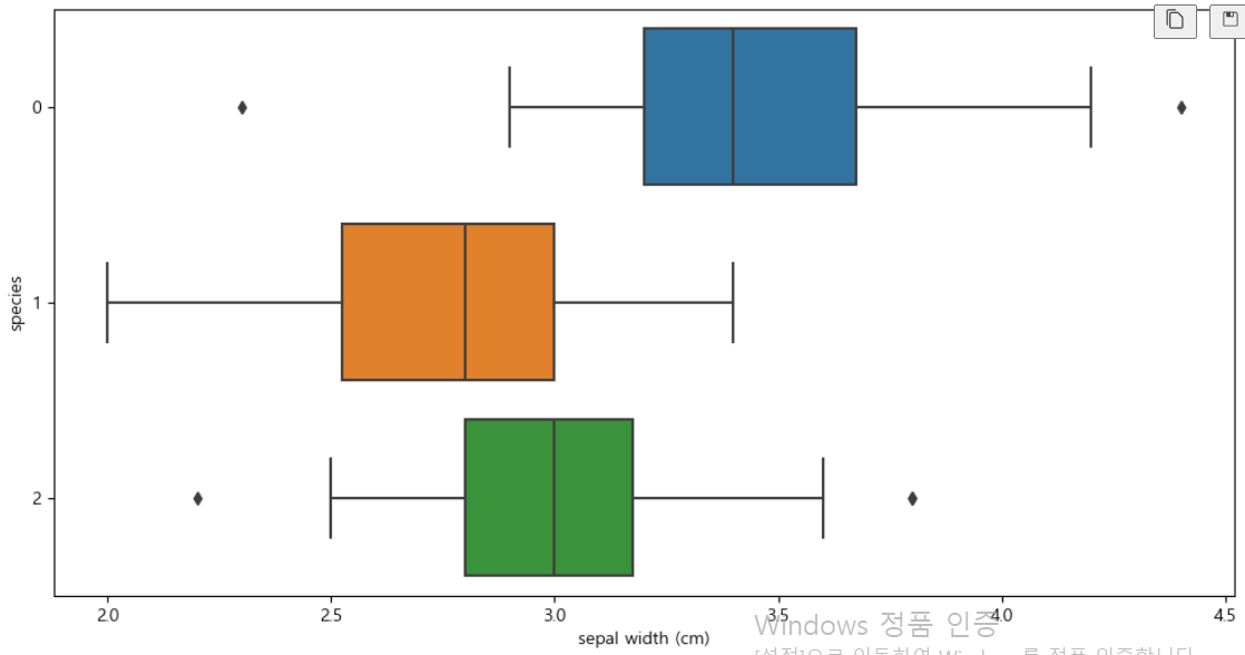
boxplot(x='sepal width (cm)')
plt.figure(figsize=(12,6))
sns.boxplot(x='sepal width (cm)', y='species', data=iris_pd, orient='h')
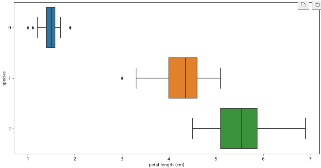
boxplot(x='petal length (cm)')
plt.figure(figsize=(12,6))
sns.boxplot(x='petal length (cm)', y='species', data=iris_pd, orient='h')
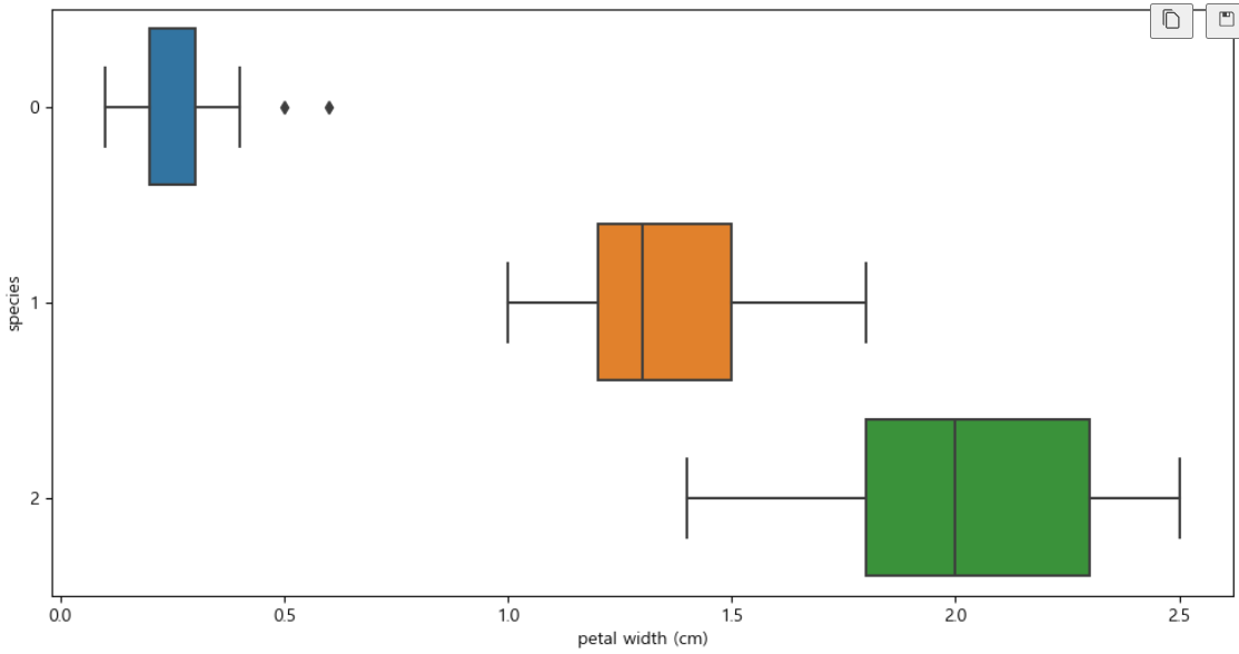
boxplot(x='petal width (cm)')
plt.figure(figsize=(12,6))
sns.boxplot(x='petal width (cm)', y='species', data=iris_pd, orient='h')
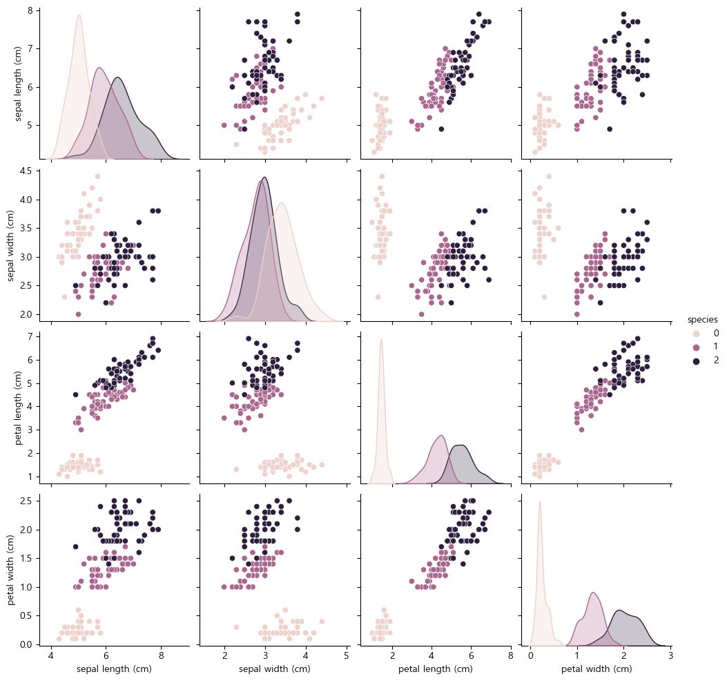
sns.pairplot(iris_pd, hue='species')
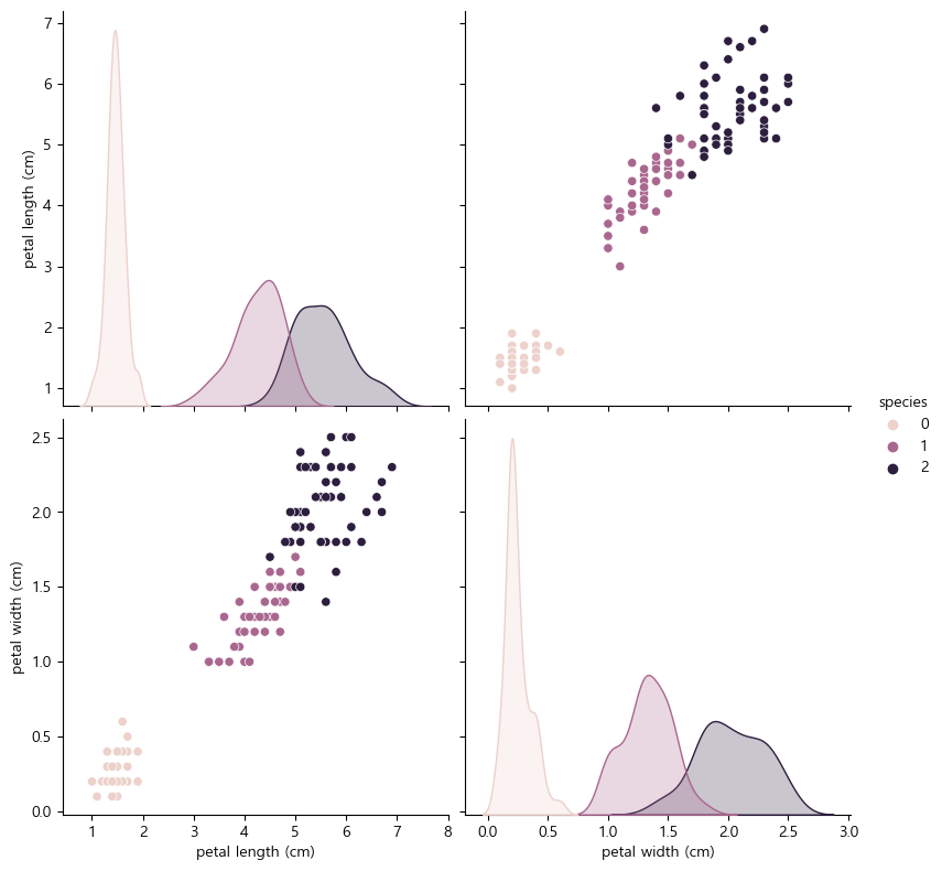
sns.pairplot(data=iris_pd, vars=['petal length (cm)', 'petal width (cm)'],
             hue='species', height=4)
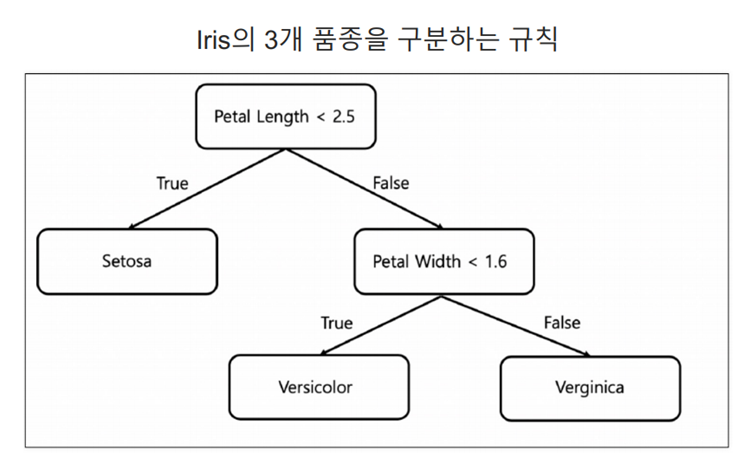
2. decision tree (결정 트리)
- 데이터의 특성(속성)에 따라 의사 결정을 내리고 그 결과를 통해 최종 예측을 수행함
Decision Tree의 분할 기준
- 정보 획득 imformation Gain
- 정보의 가치를 반환하는 데 발생하는 사전의 확률이 작을수록 정보의 가치는 커진다
- 정보 이득이란 어떤 속성을 선택함으로 인해서 데이터를 더 잘 구분하게 되는 것
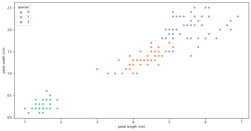
plt.figure(figsize=(12,6))
sns.scatterplot(x='petal length (cm)', y='petal width (cm)',
                data=iris_pd, hue='species', palette='Set2')
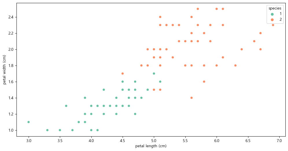
setosa는 구분이 명확하니 setosa를 제외한 두 품종만 비교하기
plt.figure(figsize=(12,6))
sns.scatterplot(x='petal length (cm)', y='petal width (cm)',
                data=iris_12, hue='species', palette='Set2')
- 엔트로피
- 얼마만큼의 정보를 담고 있는가? 무질서도를 의미, 불확실성을 나타냄
- 지니 계수
- gini index 혹은 불순도율
- 엔트로피의 계산량이 많아서 비슷한 개념이면서 보다 계산량이 적은 지니계수를 사용하는 경우가 많다
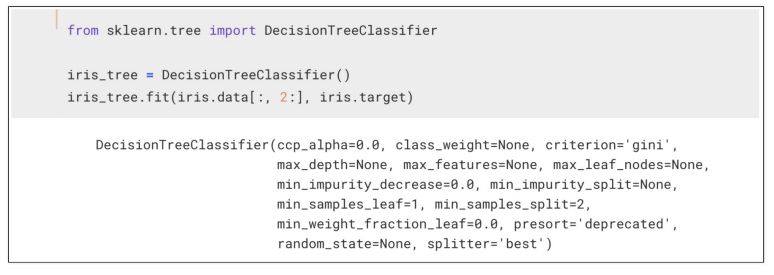
3. Scikit Learn
- 가장 유명한 기계 학습 오픈 소스 라이브러리
- DecisionTreeClassifier : 결정 트리 분류기
- fit : 학습 명령어
4. 과적합
- 지도 학습
- 학습 대상이 되는 데이터에 정답(label)을 붙여서 학습 시키고 모델을 얻어서 새로운 데이터에 모델을 사용해서 ‘답’을 얻고자 하는 것
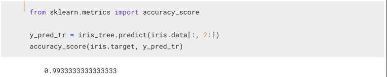
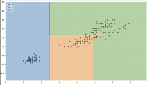
결정 경계 확인해보기
!pip install mlxtend
from mlxtend.plotting import plot_decision_regions
plt.figure(figsize=(14, 8))
plot_decision_regions(X=iris.data[:, 2:], y=iris.target, clf=iris_tree, legend=2)
plt.show()
accuracy이 높지만 경계면이 올바른지 확인할 필요가 있다.
5. 데이터 분리
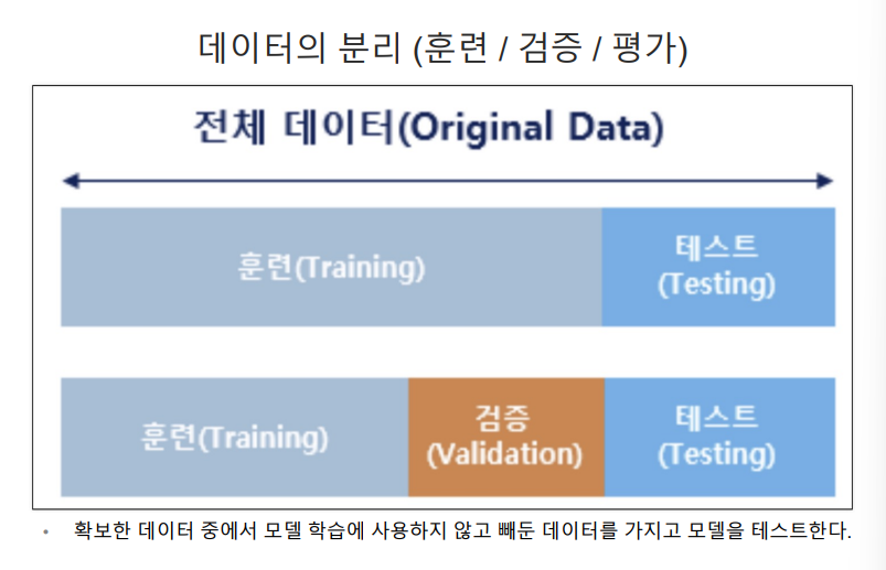
훈련용, 테스트용으로 분리하기
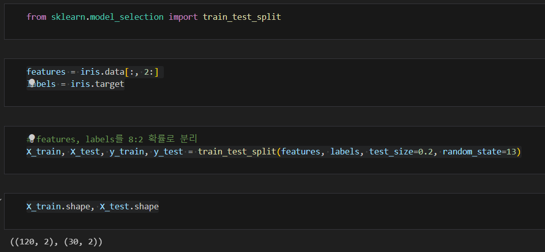
잘 분리 되었는지 확인
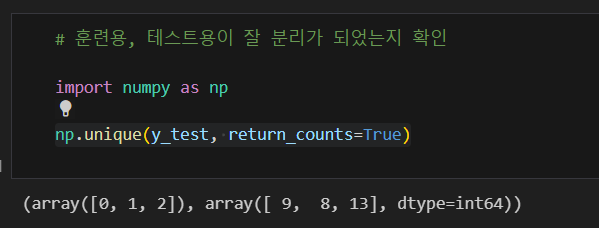
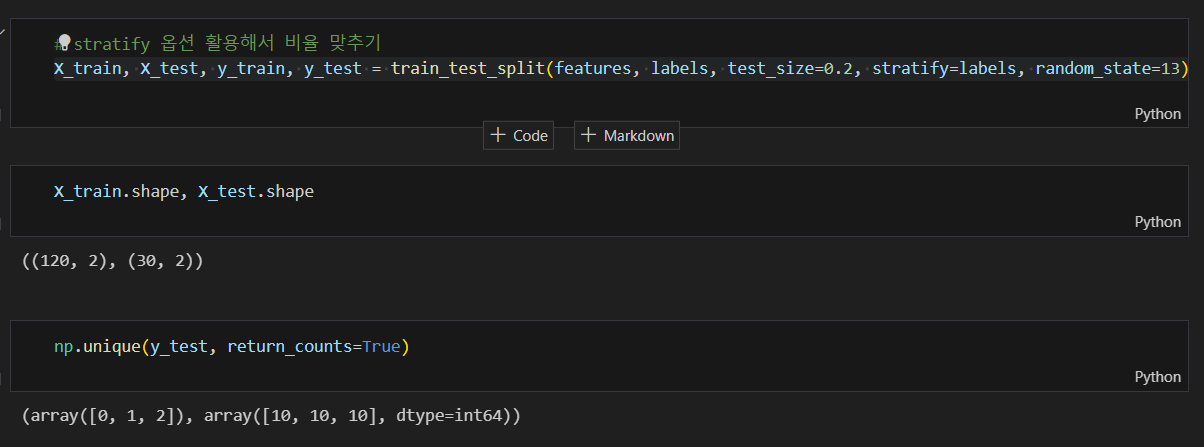
각 클래스 별 동일한 비율로 나눠지지 않아 srratify 옵션 사용하여 비율 맞추기
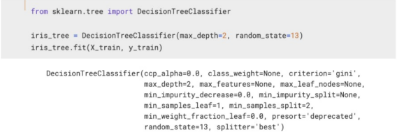
train 데이터만 대상으로 결정트리 모델 만들기
- random_state : 호출할 때마다 동일한 학습/테스트용 데이터 세트를 생성하기 위해 주어지는 난수 값.
- max_depth : 모델을 단순화시키기 위해 조정 (성능 낮아짐)
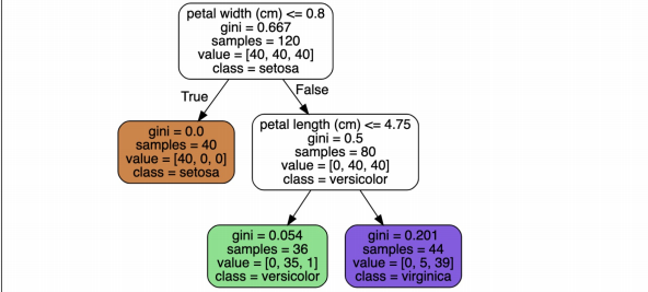
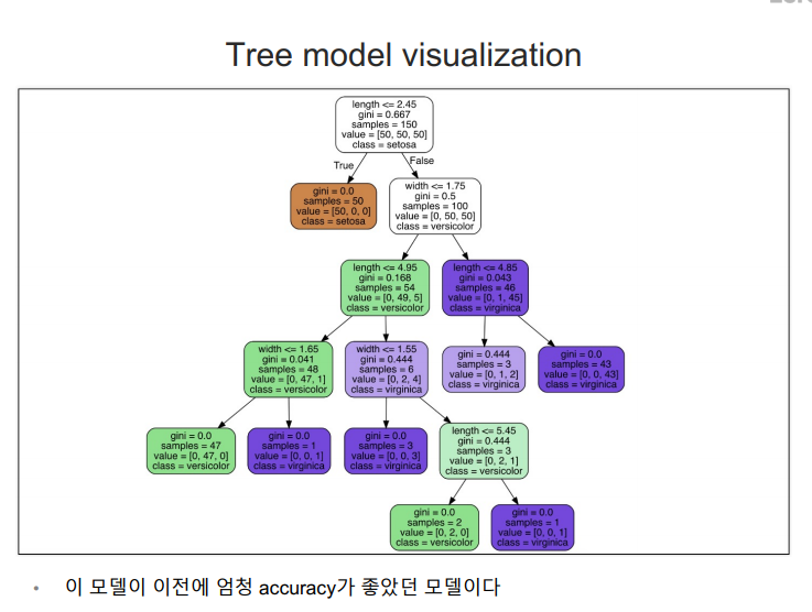
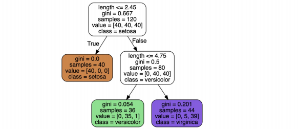
결정나무 모델 확인하기
from sklearn.tree import plot_tree
plt.figure(figsize=(12,8))
plot_tree(iris_tree);
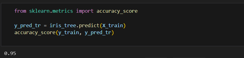
성능 확인하기
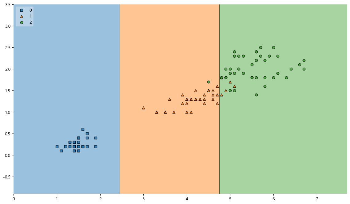
훈련용 데이터에 대한 결정경계
from mlxtend.plotting import plot_decision_regions
plt.figure(figsize=(14, 8))
plot_decision_regions(X=X_train, y=y_train, clf=iris_tree, legend=2)
plt.show()
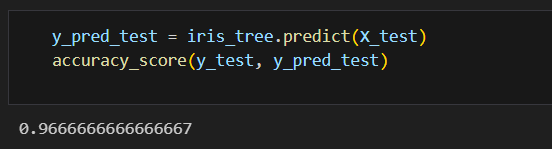
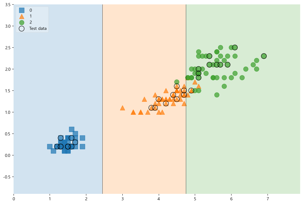
테스트 데이터에 대한 성능 확인하기
전체 데이터에서 관찰하기
scatter_highlight_kwargs = {'s' : 150, 'label':'Test data', 'alpha':0.9}
scatter_kwargs = {'s' : 120, 'edgecolor':None, 'alpha':0.7}
plt.figure(figsize=(12,8))
plot_decision_regions(X=features, y=labels,
                      X_highlight=X_test, clf=iris_tree, legend=2,
                      scatter_highlight_kwargs=scatter_highlight_kwargs,
                      scatter_kwargs=scatter_kwargs,
                      contourf_kwargs={'alpha':0.2})
plt.show()
전체 특성 학습시키기
features = iris.data
labels = iris.target
X_train, X_test, y_train, y_test = train_test_split(features, labels, test_size=0.2, stratify=labels, random_state=13)
iris_tree = DecisionTreeClassifier(max_depth=2, random_state=13)
iris_tree.fit(X_train, y_train)
전체 특성을 사용한 결정나무 모델

모델 사용 방법
- 추론
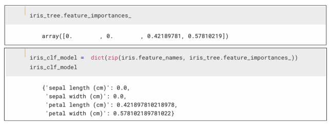
- 주요 특성 확인하기
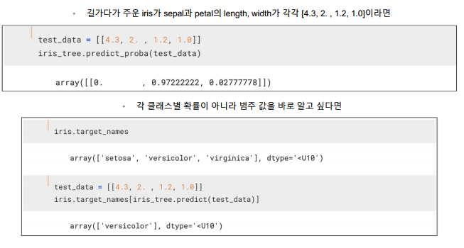
predict 함수와 predict_proba함수
predict 함수
- 각 입력 샘플에 대한 예측된 클래스 레이블을 반환
- 이진 분류 문제의 경우, 결과는 보통 0 또는1로 반환
predict_proba함수:
- 각 입력 샘플에 대해 클래스별 확률을 반환
- 반환된 값은 각 클래스에 속할 확률을 나타내며, 이진 분류에서는 보통 두 개의 확률로 구성 (클래스 0일 확률, 클래스 1일 확률)
"이 글은 제로베이스 데이터 취업 스쿨의 강의 자료 일부를 발췌하여 작성되었습니다.”

데이터 공부 기록