1. Gaussian Process Review

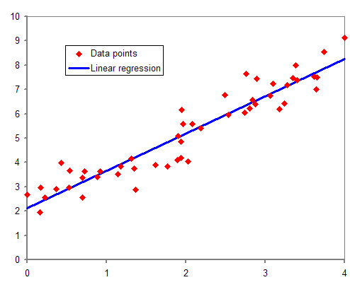
• probabilistic regression

  $y_i = f(x_i;\theta) + \epsilon_i$
  $\epsilon_i \sim N(0, \sigma^2)$
  $y_{new} \mid x_{new};\theta_{ML} \sim N(f(x_{new};\theta), \sigma^2I )$

데이터의 분포에 맞는 f(x)를 결정(선형, 비선형 모델).
가정한 모델의 parameter를 최적화.
true model(f(x))에서 관측오차를 포함한 형태로 데이터가 생성됨을 가정한 모델.

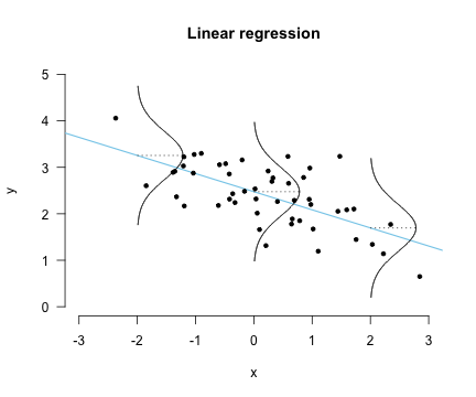
• bayesian regression

$\theta \sim p(\theta)$
$p(\theta \mid y, X) = {p(y\mid X, \theta)p(\theta)\over p(y\mid X)}$
$p(y_{new} \mid x_{new},X,y) = \int p(y_{new}\mid x_{new}, \theta)p(\theta \mid X,y)d\theta$

모델의 파라미터도 random variable로 다룬다.
data의 정보를 통해 구한 parameter의 posterior 분포를 이용해 point estimation의 형태가 아닌 분포의 형태로 estimation을 진행한다.

data uncertainty(observation noise)와 model uncertainty(parameter uncertainty)를 모두 고려함.

지금까지의 방식은 모두 f(x)의 형태를 가정한 상태로 해당 모델의 parameter를 최적화하는 방식으로 진행됨.
같은 데이터라도 여러 f(x)를 가정하고 모델링이 가능하다.
어떤 것이 최적의 모델인지는 알기 힘들다(bias-variance trade off by complexity)

f(x)를 바로 추정할 수 없을까?(priors over function space)
->function space를 다루기도 힘든데, 확률 값을 부여하기는 더욱 힘들 것이다.

따라서 function을 보다 쉽게 다루기 위해서 이를 무한 차원의 벡터로서 생각해보자.

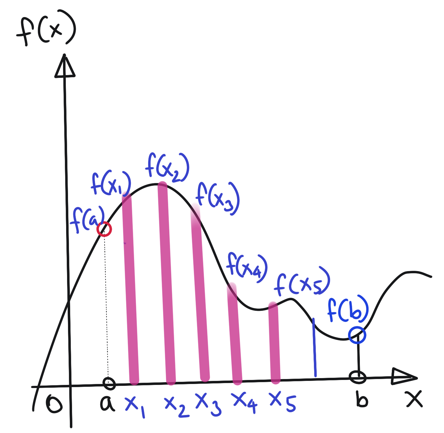
따라서 function에 prior를 부여하는 것은 무한차원의 벡터에 prior를 부여하는 것 -> 무한개의 확률 변수들로 이루어진 벡터로 표현될 것이다.(random process)

random process는 어떻게 characterize하는가-어떻게 특성을 부여하는가? (확률변수는 분포함수를 이용해 characterize된다.)

$(x_1, x_2, ...x_n) \sim p(f(x_1),f(x_2)...,f(x_n))$
joint distribution을 이용해 characterize -> joint distribution이 mutivariate gaussian -> gaussian process

$input = (x_1, x_2, ...x_n)$

$f\sim GP(\mu,K)$

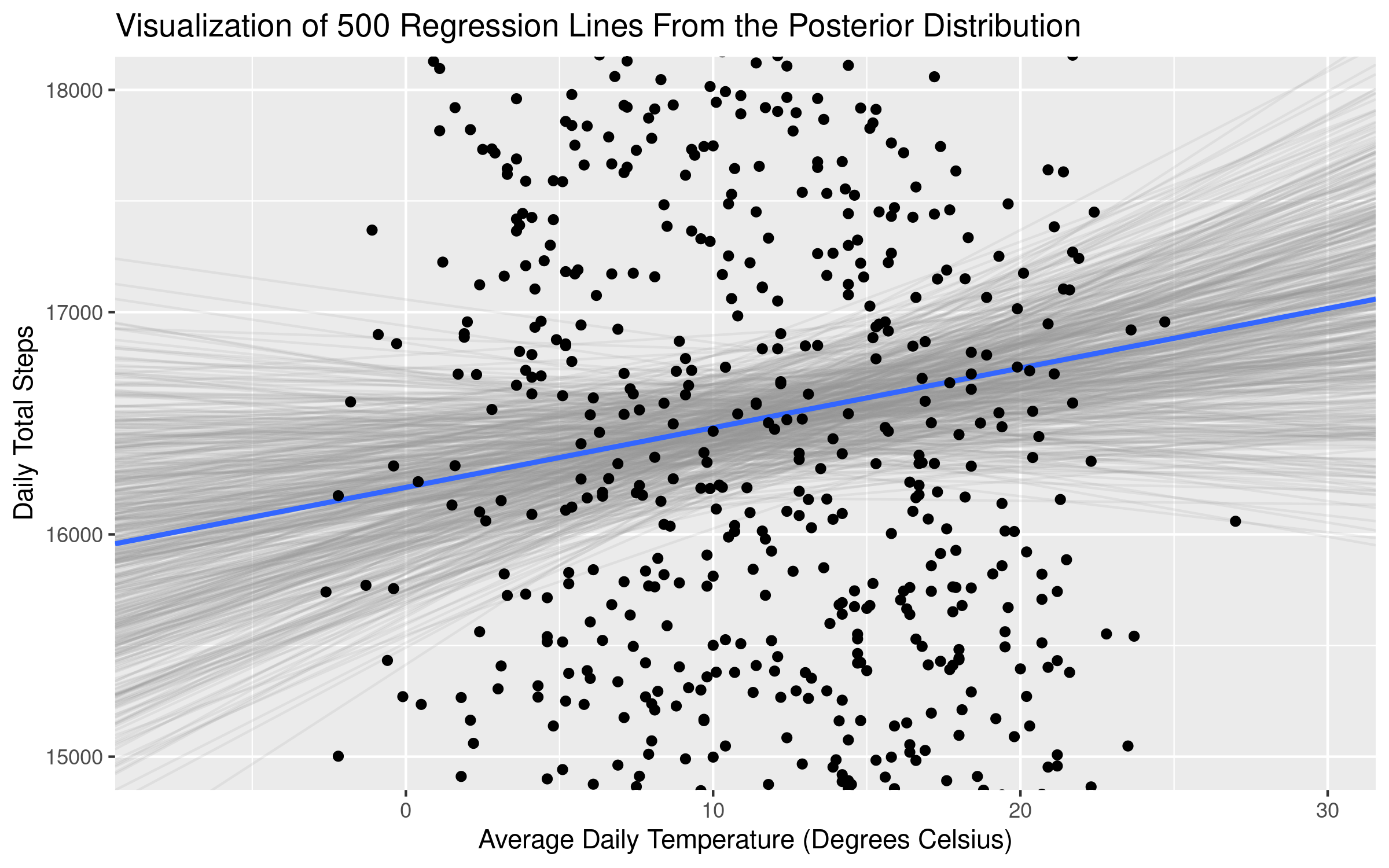
그렇다면 새로운 데이터가 관측되었을 때, f의 posterior는 어떻게 구하는가

$f\sim GP(0,K)$
$p(f_n)=N(f_n\mid 0,K_{nn})$
$p(f_{new}(x_{new})\mid f_n)=N(f_n\mid 0,K_{nn})$

multivaritate normal의 성질과 GP의 성질을 이용하여 계산

• gaussian process regression

  $f\sim GP(0,K)$
  $y(x_i):=y_i=f(x_i)+\epsilon_i$
  $f_n \sim N(f_n\mid 0,K_{nn})$
  $y\sim N(0, K_{nn}+\sigma^2I_n)$
  $y\sim GP(0, K_{nn}+\sigma^21_{x=x'})$

function의 prior로부터 뽑아낸 것과 추가적인 관측오차가 포함된 모델

pros&cons

• gaussian processes are universal function approximator
• closed posterior
• simple hyperparameter tuning
• high cost
• need to specify kernel function

2. Neural Process

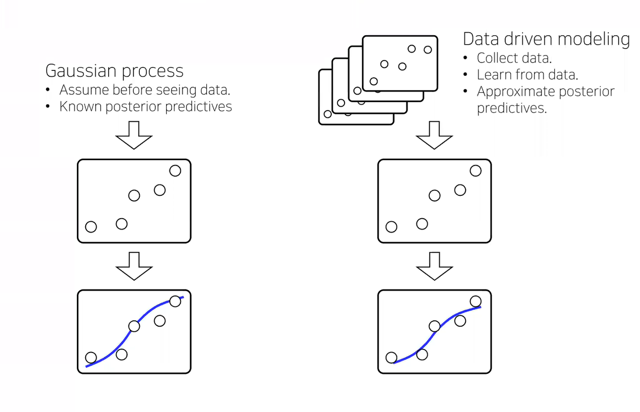
gaussian process는 이론적으로 universal function approximator이지만, 현실에서는 데이터가 충분히 주어지지 않은 경우가 대다수이다. 또한 kernel의 선택에 민감하다. -> GP가 잘 되길 바라는 경우가 대다수(주어진 데이터의 상황에서 GP를 맞추는 형식)

best random process is not necessarily a GP
-> approximate best random process(data driven modeling)
(반대로 데이터에 맞춰 random process를 추정하자)

• Using neural networks to construct stochastic processes(random functions)
• A type of 'implicit' stochastic processes
  (SP의 분포는 신경쓰지 않겠다.)
  $f(x) = g(x,z;\theta),z\sim p(z)$
  g: deterministic transformation with neural net
  z: randomness from noise distribution
  determinitic한 function에 randomness추가 -> random function

$y= f(x)+\epsilon(x), f\sim ???, \epsilon(x)\sim N(0,\sigma^2(x))$
$p(y_{new}\mid X,y)=p(y_{new}\mid NN(x_{new},X,y;\theta))$

heteroscedastic errors(input에 따라 관측오차가 달라짐(GP에서도 불가능한 가정은 x)->보통 이것도 NN이용)
implicit function prior
construct posterior predictive with neural net
(prior에대한 계산 없이 바로 NN이용해 posterior predictive 구현)

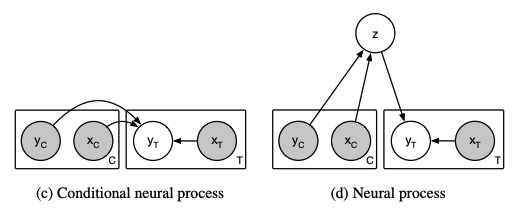
3.conditional Neural Process

• The simples version of neural processes
• 사실 이게 더 먼저
• 엄밀하게는 stochastic process가 아니다.
• NP는 CNP의 확률적인 version(vae-ae관계, z:random variable->mean,std 모델링-> r isn't deterministic)
  

$p(y_{new} \mid NN(x_{new},X,y_n;\theta)) = N(y_{new}\mid \mu(x_{new},r), \sigma^2(x_{new},r))$
$r = g_{enc}(X,y)$
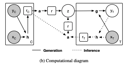
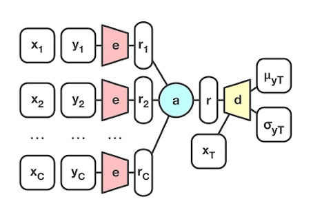
neural new encoding the set(X,y) into vector
mu,sigma is neural net

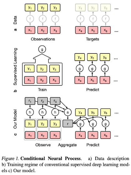
h를 이용해 각각의 함수들 ri를 찾는다.
여기서의 ri가 stochastic process의 근사값.
다음 각각의 ri를 합쳐 하나의 r을 만든다.
그러나 r은 deterministic하기 때문에 functional uncertainty에 대한 모델링은 없다.

• neural process
  reparametrization trick을 이용해 r에 randomness를 가한다. (functional uncertainty)