작성자 : 권오현

Abstract

Neural Speech Synthesis 모델들은 Text-to-Speech 와 compression applications을 위한 high quality 읍성 합성이 가능한 것을 입증했다. 이러한 새로운 모델들은 real-time operation을 위해 powerful GPUs가 필요한데, WaveRNN을 변형하여 Linear Prediction과 recurrent neural networks를 결합한 LPCNet을 제안함으로써 WaveRNN보다 훨씬 더 높은 퀄리티의 Speech synthesis가 가능하며, 3GFLOPS보다 낮은 complexity로 embedded systems나 mobile phones와 같이 lower-power devices에 deploy할 수 있음

FLOPS : 초당 부동소수점 연산, 컴퓨터가 1초동안 수행할 수 있는 부동소수점 연산의 횟수를 기준으로 삼는다.
ex) GPT-3의 사전 학습에 필요한 계산은 3640 petaflop/s-day ( 24시간동안 초당 $10^{15}$(1000조)개의 부동소수점 연산을 수행하는데 소요되는 전력

Introduction

• Neural Speech synthesis 모델은 최근에 high-quality speech synthesize와 code high quality speech at very low bitrate

• WaveNet 기반의 알고리즘들은 high-end GPU를 통해서만 real-time operation이 가능하기 때문에 end-user devices( ex. mobile phones)에서 사용불가

$\rightarrow$ 논문 저자들은 speech synthesis를 end-user devices에서 사용할 수 있게 하고자 함 (No powerful GPUs, Limited battery capacity)

• FFTNET, WaveRNN 같은 모델들은 speech synthesis의 complexity를 줄이기 위해 노력함

• Low bitrate vocoders와 같은 Low complexity parametric synthesis models이 존재함

  • quality가 제한적이며, Linear Prediction을 사용하여 음성의 spectral envelope(vocal tract response)를 모델링 하는데 효율적이지만 excitation signal을 모델링 하는데 문제가 있음

    Spectral envelope : 스펙트럼 포락선, 발음마다 vocal tract의 구조가 달라 주파수의 증폭과 감쇠가 달라짐, 발음의 종류를 결정하는 주요한 특징
    excitation signal : 여기 신호, 유성음(여러 배음들로 스펙트럼 구성), 무성음(백색소음과 같은 스펙트럼)

$\rightarrow$ 저자들은 spectral envelope modeling을 neural synthesis network를 사용하지 않은 model을 제안하여 complexity를 줄이면서 SOTA모델과 동일한 quality를 보장하는 방법을 제안하였다.

WaveRNN

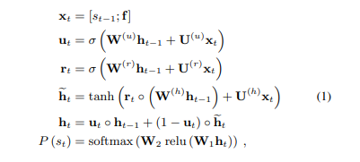
• WaveRNN은 이전 Audio Sample인 $s_{t-1}$과 conditioning parameters $f$를 통해 discrete probability distribution인 Output Sample $P(s_t)$를 생성함

• RNN(GRU) + Two fully-connected layers이 연결된 dual softmax layers로 구성되어 있으며, WaveNet과 비교하여 학습된 모델 사이즈가 작으며 speech synthesis가 빠름

• 16-bit model(8 coarse bits(=high bits) and 8 fine bits(=low bits)) $\rightarrow$ 8 corarse bits를 먼저 예측하고, 이를 기반으로 8 fine bits를 예측하여, 16-bits sample을 예측하는 것이 아닌 8-bits sample을 두개 예측하여 complexity가 낮음

$\rightarrow$ LPCNet의 경우 coarse/fine split을 생략

• $W^{(·)}, U^{(·)}$ 는 GRU weights, complexity를 줄이기 위해 GRU weights matrix를 4x4 or 16x1 non-zero block을 사용하여 spase하게 구성했음

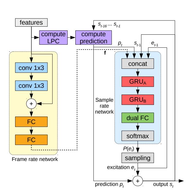
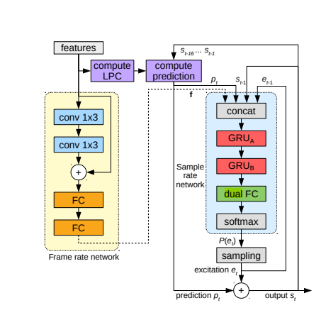
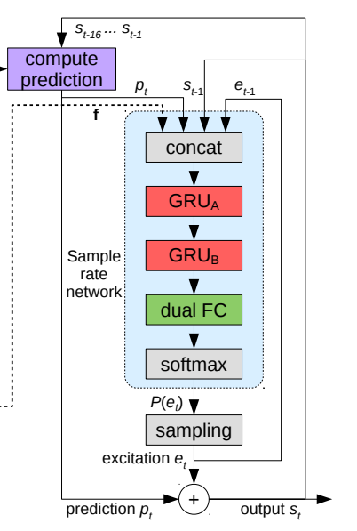
LPCNet

• 16kHz을 연산하는 sample rate network와 10-ms frames(160개의 sample, =100FPS)을 처리하는 frame rate network로 구성되어 있다

• 논문에서는 Audio input을 20 features로 제안하여 연구를 진행하엿다

  • 18 Bark-scale cepstral coefficients, 2 pitch parameters(period, correlation)

Conditioning Parameters

• Frame rate network에서 Audio의 20features가 two convolution layers(filter size =3, conv 3x1)을 통해 5 frame의 receptive field가 되어 residual connection과 two fully-connected layers를 통과하여 128-dimensional conditioning vector $f$ 가 되어 sample rate networks의 conditioning vector $f$ 가 된다

Pre-emphasis and Quantization

• WaveNet과 같은 synthesis model은 output sample values를 256으로 줄이기 위해 8-bit $\mu$-law quantization을 사용한다

• Speech signals의 대부분은 low frequencies에 집중되는 경향이 있기 때문에, $\mu$-law white quantization noise는 high frequencies에서 들을 수 있다
  $\rightarrow$ 이러한 문제를 해결하기 위해 16bits로 quantization (ex. Audio CD)을 하는 경우가 많다

• 위의 문제를 해결하기 위해 논문 저자들은 first-order pre-emphasis filter를 training data에 적용하였다

  • pre-emphasis filter : $E(z) = 1-\alpha z^{-1}$, high frequencies에 대한 noise의 영향을 줄이기 위해 frequencies를 강화시켜 high frequencies의 noise 영향을 줄이는 방법
    $\rightarrow$ synthesis의 output에 대해서는 inverse(de-emphasis) filter를 적용하여 noise를 줄일 수 있었으며, 8-bit $\mu$-law output이 high-quality synthesis에 성공할 수 있도록 만든다

Linear Prediction

• Neural speech synthesis approaches는 glottal pulses, noise excitation, vocal tract response를 포함한 speech production process를 modeling 해야 한다

• vocal tract response의 경우 all-pole linear filter를 통해 표현될 수 있다 (all-pole = autoregressive, AR, 자기회귀)

  • vocal tract를 필터로 본다면 필터의 coefficients를 구할 수 있으며, 이를 음성의 특징을 짓는 시스템으로 생각할 수 있다

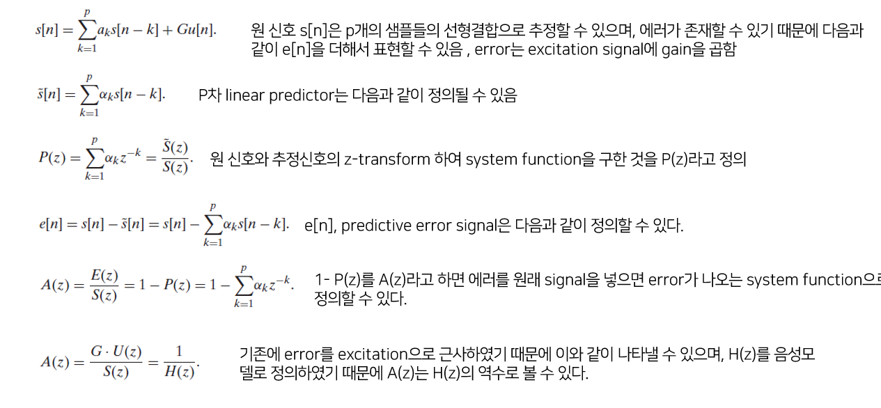
  • $s_t$를 time t의 signal로 생각하면, 이것의 linear prediction을 이전 샘플들을 기반으로 보았을 때 다음과 같이 생각할 수 있다
    

  • $a_k$는 현재 frame을 위한 $M^{th}$ order linear prediction coefficients (LPC)로 볼 수 있다

  • $a_k$를 구하는 방법 :

    

    

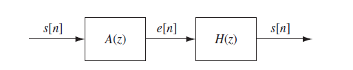
  • 위의 식을 정리해보면 음성신호가 prediction error filter A(z)를 통과하면 excitation을 추정하는 error signal이 나오게 되며, 이러한 error signal이 vocal tract response model H(z)를 통과하면 음성신호가 된다
    

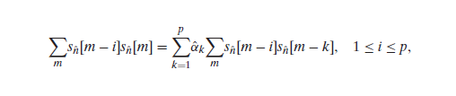
  • 이러한 모델의 장점은 vocal tract를 all-pole model 식으로 하여 LP coefficient를 찾으면 되는 장점이 있음 -> $s ,\tilde{s}$ 사이의 제곱으로 error function으로 정하여 최소화 하는 $a_k$를 찾으면 된다
    

  • 위의 식을 미분하면 다음과 같이 나온다
    

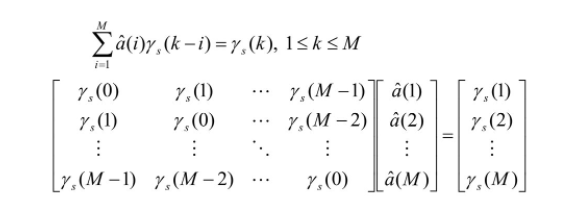
  • all-pole model이기 때문에 correlation으로 정리하여 matrix로 표현하면 다음과 같이 구할 수 있으며 쉽게 $a_k$를 구할 수 있다
    
    

• Prediction coefficients $a_k$를 계산하기 위해 18-band Bark-frequency ceptrum을 linear-frequency power spectral density(PSD)로 변환하여 계산해야 한다

  • PSD는 Inverse FFT를 사용하여 auto-correlation으로 표현할 수 있으며 Levinson-Durbin algorithms을 통해 쉽게 Predictor의 coefficients $a_k$를 구할 수 있다.

• Cepstrum으로 부터 구해진 Predictor는 speech coding text와 같은 additional information 또는 synthesize가 필요하지 않는다.

• LPC Analysis는 cepstrum이 low resolution하기 때문에 input signal 만큼 정확하지는 않지만, network가 이러한 부분까지 학습할 수 있기 때문에 출력에 미치는 영향이 적다.

  • WaveNet을 이용하여 vocal tract를 모델링 하려고 한 GlotNet의 open-loop filtering approaches보다 장점이 있다고 하였다.

• Linear Prediction을 사용하여 neural network에 영향을 주어, network가 sample values를 예측하는 것이 아닌 excitation (prediction residual)을 예측하도록 도울 수 있다.

  • 이는 network가 더 쉽게 예측을 할 수 있으며, 일반적으로 excitation이 pre-emphasized signal보다 작은 amplitude를 가지기 때문에 $\mu$-law quantization noise를 감소시킬 수 있다.

• 즉, network 이전에 sampling된 excitation $e_{t-1}$뿐만 아니라 과거 신호 $s_{t-1}$, current prediction $p_t$를 input으로 받아 더 좋은 성능을 낼 수 있다.

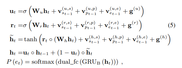
Output Layer

• Output Probabilities를 계산을 쉽게 하기 위해 two fully-connected layers을 경합한 dual_fc layers를 정의하였다. (element-wise weighted sum)
  
  
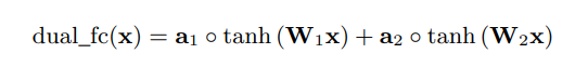
• dual fully-connected layer는 필수적인 요소는 아니지만 동일한 복잡도의 fully-connected layer와 비교 했을 때, output의 quality를 향상시킨다는 것을 발견했습니다.

Sparse Matrices

• 모델의 complexity를 낮추기 위해 저자들은 Largest GRU를 위해 일반적인 GRU(element-by-element sparseness) 대신에 WaveRNN에서 사용한 Block-sparse matrices를 사용하였다.

• Training은 dense matrices로 시작하지만, 원하는 sparseness가 달성될때까지 magnitude가 가장 낮은 block을 0으로 만들어 vectorlization을 쉽게 하도록 하였다. (16x1 blocks가 우수한 성능을 제공하였다.)

Embedding and Algebraic Simplifications

• 일반적으로 sample values를 network의 input으로 하기전에 고정된 범위로 scaling을 하지만 논문 저자들은 $\mu$-law values의 discrete한 특성을 통해 embedding matrix E를 학습하여 embedding을 하였다.

  • Embedding은 각각의 $\mu$-law level을 vector에 매핑하여, $\mu$-law value에 적용될 non-linear function set을 학습한다. 그결과 embedding matrix를 시각화 하였을때, embedding matrix E $\mu$-law scale을 linear하게 변환하는것을 알게 되었다.

• sample values를 embedding한 값들을 GRU의 input으로 넣지 않고 GRU의 non-recurrent weights $U^{(·)}$의 submatrices와 pre-computing 하여 complexity를 감소하였다 .

  • $U^{(u,s)}$를 sample $s_{t-1}$의 입력 sample의 embedding에 적용되는 columns로 구성된 $U^{(u)}$의 submatrix라고 하면, sample $s_{t-1}$을 update gate의 non recurrent 항에 직접 매핑하는 새로운 embedding matrix $V^{(u,s)}$ = $U^{(u,s)}E$로 표현할 수 있다.

  • 모든 게이트 $(u,r,h)$ 및 모든 입력 $(s,p,e)$에 대해 pre-computed된 $V^{(·,·)}$로 표현할 수 있다. $g^{(·,·)} = U^{(·)}f$

  • frame conditioning vector $f$ 또한 input의 entire frame에 대해 일정하기 때문에 위와 같은 방법으로 단순화 할 수 있다.

    $\rightarrow$ 이러한 단순화를 통해 GRU의 모든 non-recurrent inputs의 cost를 무시하여 complexity를 낮출 수 있다.
    

Sampling from Probability Distribution

• Output Probability distribution $P(e_t)$에서 직접 sampling을 하게 되면 excessive noise가 발생할 수 있다. 이것은 FFTNET 제안한 방법으로 상수 $c=2$를 곱하여 해결할수 있지만, 논문 저자들은 이러한 binary voicing decision을 만드는 대신에 $c = 1 +max(0,1.5g_p-0.5)$ 를 제안하여 문제를 해결하였다. ($g_p$ : pitch correlation)

• 위의 방법을 통해 Probability distribution를 다음과 같이 정의하였다.
  

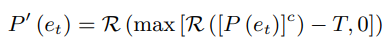
  • $\mathcal{R}(·)$ operator는 분포들을 다시 정규화

• 논문 저자들은 $T = 0.002$ 일때 impulse noise을 줄이는것과 speech가 자연스러움의 trade-off중 좋은 성능을 보인다고 하였다.

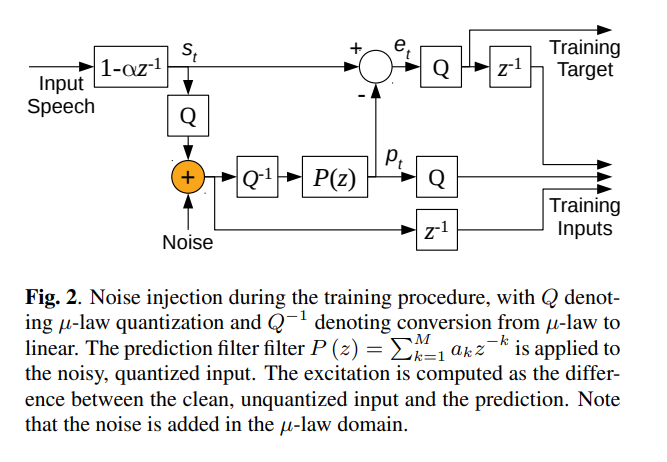
Training Noise Injection

• Speech를 synthesizing 할때, Network는 생성된 샘플이 훈련 중 사용된 샘플과 다르므로 불완전하다.

• 이러한 mismatch는 synthesis에서 excessive distortion을 야기할 수 있어 mismatch에 robust하게 만들기 위해 noise를 input에 추가하여 학습을 진행했다.

• Linear Prediction을 사용하면 noise-injection이 중요한데, signal에 noise를 추가하여 학습을 하면 noise가 synthesis filter 와 같은 형태를 갖는 pre-analysis-by-synthesis vocoder era와 유사한 artifacts를 생성하는것을 확인하였다.
  

• noise를 추가함으로써 network가 signal domain의 error를 최소화하는 것을 효과적으로 학습하는것을 확인했다.
  $\rightarrow$ network의 output은 prediction residual 이지만 input중 하나는 residual을 계산하는데 사용된 것과 동일하게 예측하기 때문에, CELP에서 제시한 analysis-by-synthesis 효과와 유사하며, synthesized speech의 artifacts를 크게 감소 시킨다.

• noise를 설정할 때, signal amplitude에 비례하도록 하기 위해 $\mu$-law domain에 직접 추가하였으며, $[-3,3]$ 범위의 uniform distribution으로 설정하였다.

EVALUATION

Complexity

• LPCNet의 complexity는 two GRUs와 dual fully-connected layer로 이루어져있다.
  

• $N_A,N_B$ : GRUs의 size, $d$ : density of the sparse GRU, $Q$ : number of $\mu$-law level, $F_s$ ; sampling rate

• $N_A = 384, N_B=16,Q=256,F_S=16000$ 로 설정했을때 약 2.8GFLOPS의 complexity를 가짐( biases, conditioning network, activation-function, $...$는 약 0.5GFLOPS의 complexity)

• 그 결과 Apple A8(Iphone 6)의 single core로 real-time synthesis를 가능하게 함 (Iphone 6S정도 되야 잘된다고 하네요..)

• WaveNet보다 작은 complexity를 가진다고 한 FFTNET의 경우 약 16GFLOPS, WaveRNN의 경우 10GFLOPS, SampleRNN의 경우 50GFLOPS complexity를 가진다고 한다

Experimental Setup

• speaker-depedent or speaker-independent 중 더 어려웅 speaker-independent에서 평가를 하였다.

• Training data는 NTT Multi-Lingual Speech Database for Telephonometry (21 languages)의 4시간 speech로 이루어져 있다.

• 120 - epochs, 64 - batch size, 각각의 sequence는 15 10-ms frames로 구성되어 있다.

• AMSGrad optimization, step_size = $\alpha = \frac{\alpha_0}{1+\delta·b}$ , $\alpha_0$=0.001, $\delta$= 5x$10^{-5}$, $b$ = batch number

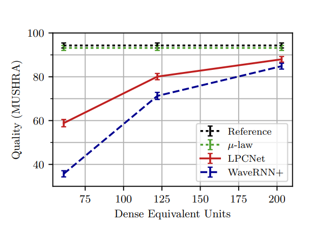
• $GRU_A$의 size 192, 384, 640 non-zero density $d =0.1$ (GRUs의 size 61,122,203이랑 동일), $GRU_B$의 size 16으로 하여 LPCNet과 WaveRNN+와 비교하였다.

Quality Evaluation

• subjective listening test인 MUSHRA를 통해 성능 비교를 하였다. (8 utterances , 2 male and 2 females speakers에 대해 100명에 의해 평가되었다.)

• LPCNet이 WaveRNN+보다 좋은 Quality를 내는것을 확인했다. 이를 통해 pre-emphasis가 $\mu$-law quantization의 noise를 무시할 수 있고, 256-value distribution(8-bit)으로 계산할 수 있기 때문에 16-bit의 WaveRNN보다 complexity가 감소한다
  

Conclusion

• LPCNet은 neural synthesis techniques와 traditional technique인 linear prediction을 결합하여 speaker-independent speech synthesis 성능이 좋은것을 확인했다.

• WaveRNN과 LPC를 단순히 결합하는거 외에도 signal values embedding, pre-emphasis와 같은 다양한 방법이 synthesis에 영향을 준다는 것을 알게 되었다.