
1주차 대회코드 : 쇼핑몰 지점별 경진대회 1차
쇼핑몰 지점별 경진대회
요약 :
- 대회 참여를 위해 Google Colab Pro 서버를 활용하여 진행했습니다.
- 데이터 분석을 하기 위해 히스토그램, 군집화, 선형성을 확인하였습니다.
- Machine Learning Model은 scikit-learn에 있는 RandomForest모델을 활용하여 가격 예측 모델을 만들었습니다.
1. 데이터 분석
- 올바른 ML Model에 학습 시키기 위해서는 정확한 데이터 분석을 해야합니다.
- 학습(Train) 데이터, 및 테스트(Test) 데이터를 불러와 학습을 합니다. 이 때 컬럼의 갯수와 이름, 타겟 데이터 등을 파악 하여 각 변수들이 어떠한 관계가 있는지 히스토그램, 히트맵, 군집화 등 다양한 데이터 분석기법을 활용하여 분석했습니다.
- 미리 요약해드리자면 각 변수간의 선형성(linearity)을 나타내는 correlation을 파악해보면 매우 낮은 값을 갖고 있다는 것을 알 수 있었고, 따라서 예측 모델을 만들기 위해서 해당 다중선형회귀 분석 및 회귀분석에는 적합하지 않음을 확인할 수 있었습니다.
1.1 패키지 다운로드
- 데이터 분석 및 ML 모델링에 필요한 패키지를 다운로드 합니다. 사용하는 라이브러니는 pandas, numpy 시각화를 위한 seaborn, matplotlib.pyplot ML 모델 학습을 위한 sklearn.model_selection의 train_test_split, sklearn.ensemble 의 RandomFroestRegressor, BaggingRegressor, DecisionTreeRegressor, AdaBoostRegressor, Xgboost를 이용해주었습니다.
# 데이터 분석
import pandas as pd
import numpy as np
# 데이터 분석(시각화)
import matplotlib.pyplot as plt
import seaborn as sns
# ML 모델링
from sklearn.model_selection import train_test_split
from sklearn.ensemble import BaggingRegressor
from sklearn.ensemble import RandomForestRegressor
from sklearn.tree import DecisionTreeRegressor
from sklearn.ensemble import AdaBoostRegressor
import xgboost
# 선형회귀
import statsmodels.api as sm
from statsmodels.stats.outliers_influence import variance_inflation_factor
# RMSE
from sklearn.metrics import mean_squared_error
.2 데이터 로드 및 Google Drive 연결
- 학습 데이터(train 데이터)와 테스트(test)데이터를 로드
- train data column
id : 샘플 아이디 Store : 쇼핑몰 지점 Date : 주 단위(Weekly) 날짜 Temperature : 해당 쇼핑몰 주변 기온 Fuel_Price : 해당 쇼핑몰 주변 연료 가격 Promotion 1~5 : 해당 쇼핑몰의 비식별화된 프로모션 정보 Unemployment : 해당 쇼핑몰 지역의 실업률 IsHoliday : 해당 기간의 공휴일 포함 여부 Weekly_Sales : 주간 매출액 (목표 예측값) - test data column
id : 샘플 아이디
Store : 쇼핑몰 지점
Date : 주 단위(Weekly) 날짜
Temperature : 해당 쇼핑몰 주변 기온
Fuel_Price : 해당 쇼핑몰 주변 연료 가격
Promotion 1~5 : 해당 쇼핑몰의 비식별화된 프로모션 정보
Unemployment : 해당 쇼핑몰 지역의 실업률
IsHoliday : 해당 기간의 공휴일 포함 여부
- train data column
• 구글 드라이브를 연결 한 뒤, 작업디렉토리로 위치를 이동합니다.
from google.colab import drive
drive.mount('/content/drive/')
cd /content/drive/MyDrive/dacon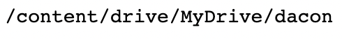
train_data = pd.read_csv("./dataset/train.csv")
train_data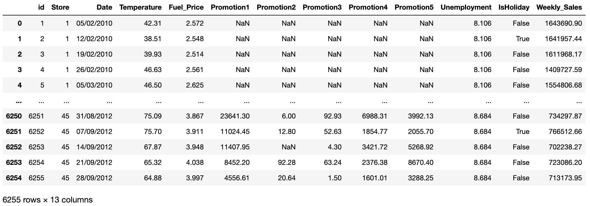
test_data = pd.read_csv("./dataset/test.csv")
test_data
1.3 데이터 전처리
- 결측치를 제거하거나(0으로 채우거나), One-hot encoding 으로 범주형 데이터를 수치형으로 변환을 하고, 정규화를 진행합니다.
- pandas에 isna()함수와 sum()함수를 활용하여 각 컬럼에 얼마나 많은 결측치가 있는지 확인하였습니다.
# 결측치 확인
train_data.isna().sum()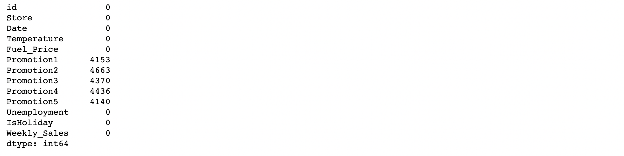
- Promotion 1~5에 Nan으로 표기된 4000개 이상입니다, 전체 데이터가 6000개정도 밖에 되지 않기 때문에 단순히 결측치를 가지고 있는 데이터를 삭제할 경우 학습데이터가 부족할 수도 있고 제대로 학습이 안될 가능성이 있기때문에 결측치는 모두 0으로 채워주도록 하겠습니다.
- 또한 Target Data인 Weekly Sales 값은 결측치가 없는 것을 알 수 있습니다.
# 결측치 0으로 채우기
train_data=train_data.fillna(0)
train_data.isna().sum()
• 값이 어떤 데이터 타입의 값이 들어가 있는지 확인해줍니다.
print(train_data.columns)
print(train_data.dtypes)
print("행 열 :", train_data.shape)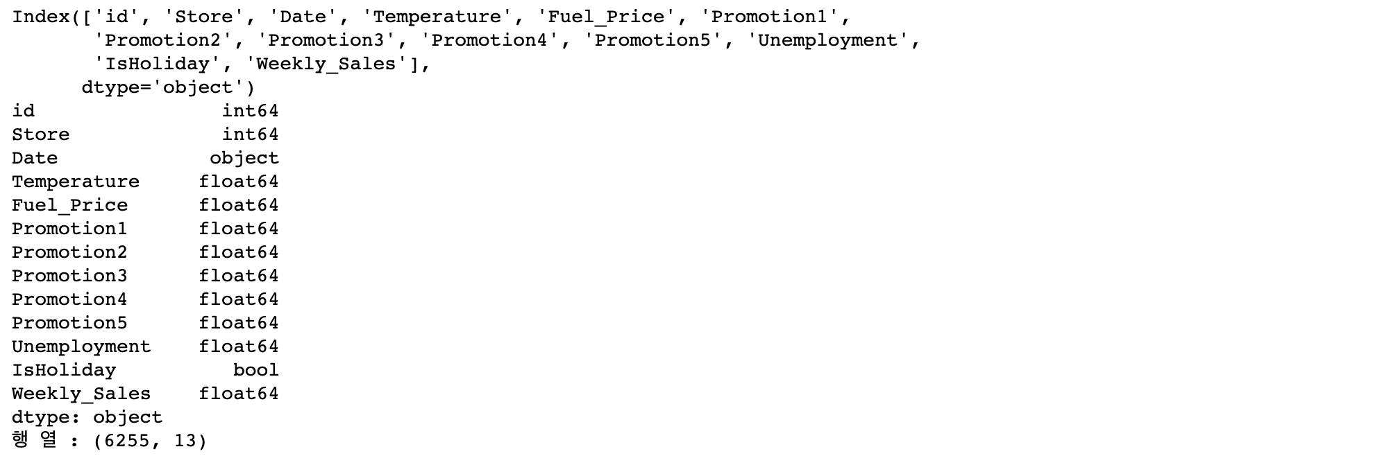
• Bool 변수를 one-hot encoding을 통해서 0,1값으로 바꿔줍니다.
train_data["IsHoliday"] = train_data["IsHoliday"].astype(int)• Date데이터의 연,월,일의 값이 object형태이기 때문에 값을 바꿔줍니다.
# Date데이터의 연월일을 변환
day =[]
month=[]
year=[]
for i in range(len(train_data["Date"])):
  day.append(int(train_data.iloc[i]["Date"][0:2]))
  month.append(int(train_data.iloc[i]["Date"][3:5]))
  year.append(int(train_data.iloc[i]["Date"][6:]))
train_data["day"]=day
train_data["month"] = month
train_data["year"] = year
• pandas에 자동으로 histogram을 만들어 주는 함수인 .hist를 이용해서 histogram을 만들어줍니다.
train_data.hist(figsize=(30,20))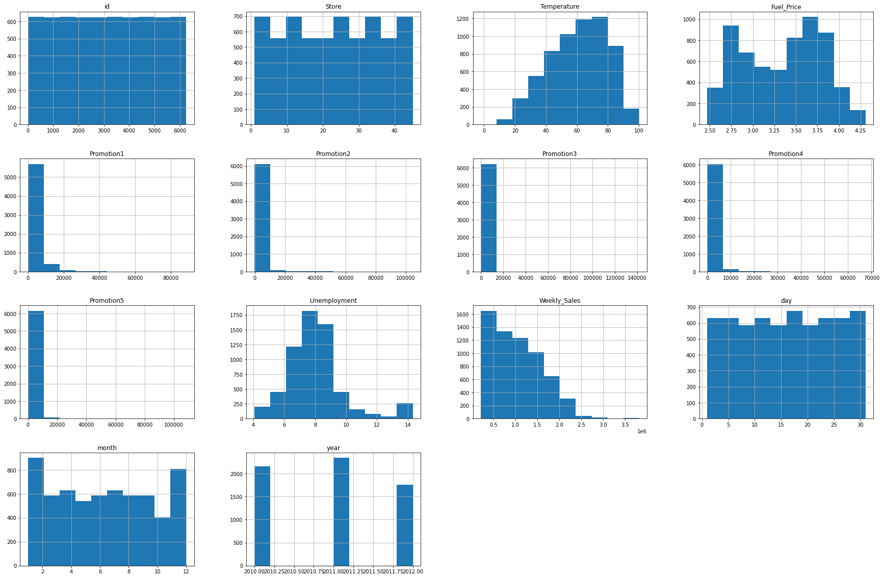
• 이제 데이터의 값의 분포를 describe함수를 통해 숫자로 확인합니다. 각 값이 mean, std, min을 살펴 분포가 어떻게 되어 있는지 파악합니다.
train_data.describe()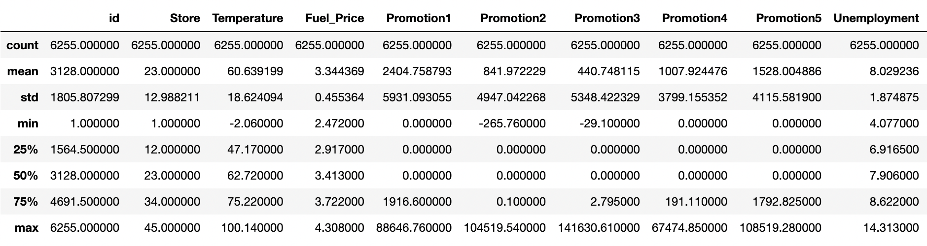
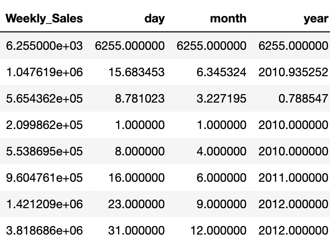
- 히스토그램과 숫자 데이터를 분석해보면 Promotion 칼럼에 해당하는 값들이 많은 값이 비워져있고 promotion1, promotion2, promotion3, promotion4, promotion5 값이 3000~5000정도이지만, 각 25%, 50% 구간이 0으로 매우 치우져있음을 알 수 있습니다. 히스토그램에서도 0에 해당하는 값들이 다른 값들보다 압도적으로 많은 것을 확인할 수 있습니다.
- 또한 Weekly_Sales의 값도 평균보다 아래의 값에 분포가 되어 있는 것을 볼 수 있습니다.
- 또한 많은 컬럼들의 숫자 범위가 크게 다른 것을 확인할 수 있습니다.
- 정규화를 적용시켜 줍니다. 정규화는 Z- 정규화를 이용할 것인데요. 데이터 분포를 통해 확인할 수 있듯이, 많은 이상치가 존재합니다. min_max를 이용할 경우 이상치에 여전히 민감하기 때문에 Z-정규화를 이용해줍니다. 분석에 활용하지 않을 id, Date 또한 Target인 Weekly_Sales를 제외한, 학습에 활용될 칼럼에 해당되는 부분을 정규화를 이용해줍니다.
# id 는 제외하고 정규화 진행
norm = train_data.drop(['id','Date', 'Weekly_Sales'],axis=1)
# z-정규화( x-평균/표준편차)
train_data_normed = (norm- norm.mean())/norm.std()
train_data_normed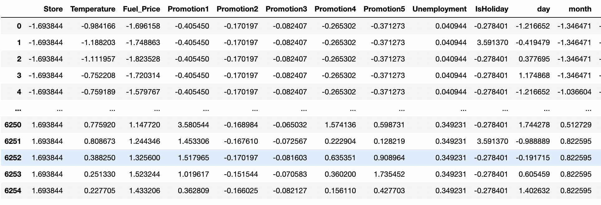
train_data_normed.hist(figsize=(30,20))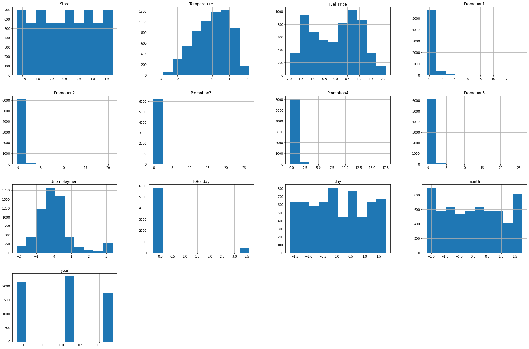
1.3 데이터 선형성(Linear Correlation)확인 - Heatmap 이용
- Target변수인 Weekly_Sales와 다른 변수와 선형성이 존재하는지 확인합니다
analysis = pd.merge(train_data_normed, train_data['Weekly_Sales'],
                left_index = True, right_index=True)
# 선형성 확인
plt.figure(figsize=(16,16))
sns.heatmap(analysis.corr(), linewidths=.5, cmap = 'Blues', annot=True)
- Weekly_Sales와 다른 변수들의 correlation을 확인해보면 store정도만 0.34의 선형성을 가지고 나머지는 0.2 이하의 선형성을 가지고 있습니다. 따라서 선형성이 높지 않기 때문에 선형회귀분석이 적합하지 않는 것을 확인하였습니다.
#pairplot with Seaborn
sns.pairplot(analysis,hue='Weekly_Sales')
plt.show()
- pairplot을 확인해보면, 특정 store들을 기준으로 값이 나눠진것을 볼 수 있습니다.
- 또한 대체로 promotion값이 높을 경우 Weekly_Sales값이 높은 것을 알 수 있습니다.
- Temperature 또한 값의 분포가 나뉘는 것을 볼 수 있습니다.
2. ML 모델링
- 선형 회귀 모델, Bagging, RandomForest, Adaboost, XGBoost모델 만들기
- 종속 변수와 타겟 데이터 설정하기
2.1 데이터 학습
- 선형성이 없는 것을 확인했습니다. 다만, 실제로 모델을 만들었을때 어느정도 RMSE 값이 나오는지 체크해보았습니다.
y_target = train_data['Weekly_Sales']
x_data = train_data_normed.drop(['Unemployment','IsHoliday','Promotion4', 'day', 'month'],axis=1)

train_x, test_x, train_y, test_y = train_test_split(x_data, y_target, train_size=0.9, test_size=0.1,random_state = 7)print(train_x.shape, test_x.shape, train_y.shape, test_y.shape)
# 임의의 변수로 초기화 뒤 학습
test_x=sm.add_constant(test_x,has_constant='add')# 상수항추가
train_x=sm.add_constant(train_x,has_constant='add')# 상수항
model = sm.OLS(train_y, train_x)
fitted_model = model.fit()fitted_model.summary()
- 다중 공산성 체크
# 다중 공산성 확인
vif = pd.DataFrame()
vif["VIF Factor"] = [variance_inflation_factor(
    x_data.values, i) for i in range(x_data.shape[1])]
vif["features"] = x_data.columns
vif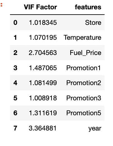
- 학습 데이터 정확도 시각화
plt.plot(np.array(fitted_model.predict(train_x)),label="pred")
plt.plot(np.array(train_y),label="true")
plt.legend()
plt.show()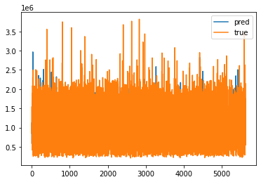
- 테스트 데이터 정확도 시각화
plt.plot(np.array(fitted_model.predict(test_x)),label="pred")
plt.plot(np.array(test_y),label="true")
plt.legend()
plt.show()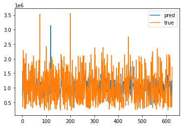
print("RMSE: ", mean_squared_error(test_y, fitted_model.predict(test_x))**0.5)RMSE: 497323.21422187285
01. Bagging을 이용한 학습
decision_tree_model = DecisionTreeRegressor()
bagging_decision_tree_model = BaggingRegressor(base_estimator = decision_tree_model, # 의사결정나무 모형
                                                n_estimators = 5, # 5번 샘플링
                                                verbose = 1, random_state=1) # 학습 과정 표시
tree_model = bagging_decision_tree_model.fit(train_x, train_y) # 학습 진행
predict = tree_model.predict(test_x) # 학습된 Bagging 의사결정나무 모형으로 평가 데이터 예측
print("RMSE: {}".format((mean_squared_error(predict, test_y)**0.5))) # RMSE 결과
RMSE: 139250.1423912945
[Parallel(n_jobs=1)]: Using backend SequentialBackend with 1 concurrent workers.
[Parallel(n_jobs=1)]: Done 1 out of 1 | elapsed: 0.1s finished
[Parallel(n_jobs=1)]: Using backend SequentialBackend with 1 concurrent workers.
[Parallel(n_jobs=1)]: Done 1 out of 1 | elapsed: 0.0s finished
02. RandomForest을 이용한 학습
for i in range(1,17):
  for j in range(100,700,100):
    RFR_model= RandomForestRegressor(n_estimators=j, max_depth=i,random_state=1)
    RFR_model.fit(train_x, train_y)
    predict = RFR_model.predict(test_x)
    print("n_estimators=",j, "max_depth=",i)
print("RMSE: {}".format((mean_squared_error(predict, test_y)**0.5)))- OUTPUT n_estimators= 400 max_depth= 8
RMSE: 184905.87504171493
n_estimators= 500 max_depth= 8
RMSE: 184688.68940690748
n_estimators= 600 max_depth= 8
RMSE: 184010.76170118622
n_estimators= 100 max_depth= 9
RMSE: 152567.9207093523
n_estimators= 200 max_depth= 9
RMSE: 151805.4567680836
n_estimators= 300 max_depth= 9
RMSE: 152555.92802593057
n_estimators= 400 max_depth= 9
RMSE: 153274.08167143856
n_estimators= 500 max_depth= 9
RMSE: 153306.42647037856
n_estimators= 600 max_depth= 9
RMSE: 152970.45832026904
n_estimators= 100 max_depth= 10
RMSE: 142441.34366849926
n_estimators= 200 max_depth= 10
RMSE: 141637.55201054775
n_estimators= 300 max_depth= 10
RMSE: 142363.17802764624
n_estimators= 400 max_depth= 10
RMSE: 143072.55846592158
n_estimators= 500 max_depth= 10
RMSE: 142757.56665801615
n_estimators= 600 max_depth= 10
RMSE: 142613.70520230802
n_estimators= 100 max_depth= 11
RMSE: 137182.4011438835
n_estimators= 200 max_depth= 11
RMSE: 136252.81978452526
n_estimators= 300 max_depth= 11
RMSE: 137159.8502322525
n_estimators= 400 max_depth= 11
RMSE: 137359.96953144704
n_estimators= 500 max_depth= 11
RMSE: 137270.77733347492
n_estimators= 600 max_depth= 11
RMSE: 137258.54276539653
n_estimators= 100 max_depth= 12
RMSE: 135880.45768915344
n_estimators= 200 max_depth= 12
RMSE: 134563.3185875039
n_estimators= 300 max_depth= 12
RMSE: 135330.89556339706
n_estimators= 400 max_depth= 12
RMSE: 135597.82068229513
n_estimators= 500 max_depth= 12
RMSE: 135545.59057905653
n_estimators= 600 max_depth= 12
RMSE: 135591.57126551442
n_estimators= 100 max_depth= 13
RMSE: 135446.72828888835
n_estimators= 200 max_depth= 13
RMSE: 134568.05784705383
n_estimators= 300 max_depth= 13
RMSE: 135265.21150808086
n_estimators= 400 max_depth= 13
RMSE: 135236.876110669
n_estimators= 500 max_depth= 13
RMSE: 135099.21528053886
n_estimators= 600 max_depth= 13
RMSE: 135132.57030176546
n_estimators= 100 max_depth= 14
RMSE: 136162.20119054237
n_estimators= 200 max_depth= 14
RMSE: 134683.7498120167
n_estimators= 300 max_depth= 14
RMSE: 135122.0344210059
n_estimators= 400 max_depth= 14
RMSE: 134854.49292357374
n_estimators= 500 max_depth= 14
RMSE: 134708.96322926308
n_estimators= 600 max_depth= 14
RMSE: 134815.00076917844
n_estimators= 100 max_depth= 15
RMSE: 134811.38347010917
n_estimators= 200 max_depth= 15
RMSE: 133806.08621948835
n_estimators= 300 max_depth= 15
RMSE: 134466.84352640525
n_estimators= 400 max_depth= 15
RMSE: 134561.82014688896
n_estimators= 500 max_depth= 15
RMSE: 134396.3583000113
n_estimators= 600 max_depth= 15
RMSE: 134559.11948637455
n_estimators= 100 max_depth= 16
RMSE: 135054.12342185475
n_estimators= 200 max_depth= 16
RMSE: 133762.48351173452
n_estimators= 300 max_depth= 16
RMSE: 134836.35265200687
n_estimators= 400 max_depth= 16
RMSE: 134867.9070369727
n_estimators= 500 max_depth= 16
RMSE: 134569.76096023954
n_estimators= 600 max_depth= 16
RMSE: 134525.255952843
03. XGboost
train_x = train_x.drop(['Promotion2','year'],axis=1)
test_x = test_x.drop(['Promotion2','year'],axis=1)
for i in range(1,10):
  for j in range(100,1000,100):
    xgb_model = xgboost.XGBRegressor(n_estimators=j, learning_rate=0.08, gamma=0, subsample=0.75, colsample_bytree=1, max_depth=i)
    xgb_model.fit(train_x,train_y)
    predict = xgb_model.predict(test_x)
    print("n_estimators=",j, "max_depth=",i)
print("RMSE: {}".format((mean_squared_error(predict, test_y)**0.5)))-
OUTPUT
n_estimators= 100 max_depth= 1
RMSE: 460015.2693717782n_estimators= 200 max_depth= 1
RMSE: 438646.87092703284n_estimators= 300 max_depth= 1
RMSE: 420736.6539690999n_estimators= 400 max_depth= 1
RMSE: 406708.72215318587n_estimators= 500 max_depth= 1
RMSE: 393728.2546447163n_estimators= 600 max_depth= 1
RMSE: 381169.74412371183n_estimators= 700 max_depth= 1
RMSE: 370252.5891072115n_estimators= 800 max_depth= 1
RMSE: 360340.88390494377n_estimators= 900 max_depth= 1
RMSE: 351164.42362712265n_estimators= 100 max_depth= 2
RMSE: 306459.3250344036n_estimators= 200 max_depth= 2
RMSE: 227511.00218503436n_estimators= 300 max_depth= 2
RMSE: 184570.61014635224n_estimators= 400 max_depth= 2
RMSE: 166715.09789379605n_estimators= 500 max_depth= 2
RMSE: 154806.26364147512n_estimators= 600 max_depth= 2
RMSE: 145513.16822728465n_estimators= 700 max_depth= 2
RMSE: 139210.25451989096n_estimators= 800 max_depth= 2
RMSE: 135226.37023649184n_estimators= 900 max_depth= 2
RMSE: 131300.71684834707n_estimators= 100 max_depth= 3
RMSE: 230008.12321863492n_estimators= 200 max_depth= 3
RMSE: 156790.0151757414n_estimators= 300 max_depth= 3
RMSE: 137698.39584197063n_estimators= 400 max_depth= 3
RMSE: 128546.74746110164n_estimators= 500 max_depth= 3
RMSE: 122741.11406964035n_estimators= 600 max_depth= 3
RMSE: 120653.50121949562n_estimators= 700 max_depth= 3
RMSE: 117548.72922108823n_estimators= 800 max_depth= 3
RMSE: 116065.74059664998n_estimators= 900 max_depth= 3
RMSE: 114153.11420794841n_estimators= 100 max_depth= 4
RMSE: 166817.01695602635n_estimators= 200 max_depth= 4
RMSE: 127788.61126348235n_estimators= 300 max_depth= 4
RMSE: 117718.12882537133n_estimators= 400 max_depth= 4
RMSE: 114488.61584448442n_estimators= 500 max_depth= 4
RMSE: 111666.8418078547n_estimators= 600 max_depth= 4
RMSE: 110229.68478890423n_estimators= 700 max_depth= 4
RMSE: 109170.83166226344n_estimators= 800 max_depth= 4
RMSE: 108568.98924373678n_estimators= 900 max_depth= 4
RMSE: 107365.36622920564n_estimators= 100 max_depth= 5
RMSE: 142063.67794971686n_estimators= 200 max_depth= 5
RMSE: 114968.18874273293n_estimators= 300 max_depth= 5
RMSE: 108744.42616551125n_estimators= 400 max_depth= 5
RMSE: 105988.58299577776n_estimators= 500 max_depth= 5
RMSE: 104290.92672024037n_estimators= 600 max_depth= 5
RMSE: 103439.03227342005n_estimators= 700 max_depth= 5
RMSE: 103046.3295739929n_estimators= 800 max_depth= 5
RMSE: 102130.05932015614n_estimators= 900 max_depth= 5
RMSE: 101592.91557067417n_estimators= 100 max_depth= 6
RMSE: 131861.4760764873n_estimators= 200 max_depth= 6
RMSE: 114358.91940001518n_estimators= 300 max_depth= 6
RMSE: 109581.71701103379n_estimators= 400 max_depth= 6
RMSE: 107599.56514532154n_estimators= 500 max_depth= 6
RMSE: 105621.65076628176n_estimators= 600 max_depth= 6
RMSE: 104761.0296357656n_estimators= 700 max_depth= 6
RMSE: 104353.59141184231n_estimators= 800 max_depth= 6
RMSE: 104003.37041523591n_estimators= 900 max_depth= 6
RMSE: 103862.50802285597n_estimators= 100 max_depth= 7
RMSE: 119340.19515015816n_estimators= 200 max_depth= 7
RMSE: 107819.72082601112n_estimators= 300 max_depth= 7
RMSE: 104259.22298844173n_estimators= 400 max_depth= 7
RMSE: 102168.19407450572n_estimators= 500 max_depth= 7
RMSE: 101106.68511514353n_estimators= 600 max_depth= 7
RMSE: 100813.9535699186n_estimators= 700 max_depth= 7
RMSE: 100810.71444835368n_estimators= 800 max_depth= 7
RMSE: 100620.56710537343n_estimators= 900 max_depth= 7
RMSE: 100355.97664846746n_estimators= 100 max_depth= 8
RMSE: 111915.80985305535n_estimators= 200 max_depth= 8
RMSE: 104762.56798154968n_estimators= 300 max_depth= 8
RMSE: 102551.65280479609n_estimators= 400 max_depth= 8
RMSE: 101987.95647842406n_estimators= 500 max_depth= 8
RMSE: 101733.19953484504n_estimators= 600 max_depth= 8
RMSE: 101581.83746708208n_estimators= 700 max_depth= 8
RMSE: 101637.00429896996n_estimators= 800 max_depth= 8
RMSE: 101587.87696639916n_estimators= 900 max_depth= 8
RMSE: 101581.70661780362n_estimators= 100 max_depth= 9
RMSE: 110798.69250859715n_estimators= 200 max_depth= 9
RMSE: 105756.71740331504n_estimators= 300 max_depth= 9
RMSE: 104304.6924234451n_estimators= 400 max_depth= 9
RMSE: 104182.49687204252n_estimators= 500 max_depth= 9
RMSE: 104174.33804807537n_estimators= 600 max_depth= 9
RMSE: 104197.34682020044n_estimators= 700 max_depth= 9
RMSE: 104243.20555470382n_estimators= 800 max_depth= 9
RMSE: 104237.35570322191n_estimators= 900 max_depth= 9
RMSE: 104263.23627733768
xgb_model = xgboost.XGBRegressor(n_estimators=500, learning_rate=0.08, gamma=0, subsample=0.75, colsample_bytree=1, max_depth=10)
xgb_model.fit(train_x,train_y)
predict = xgb_model.predict(test_x)
print("RMSE: {}".format((mean_squared_error(predict, test_y)**0.5)))
RMSE: 104132.56244340152
xgboost.plot_importance(xgb_model)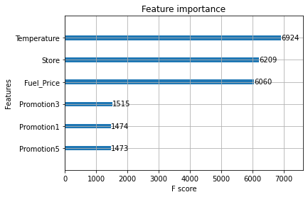
04. AdaBoost Regressor
for j in range(100,1000,100):
  Adaboost_model = AdaBoostRegressor(n_estimators=j,random_state=1)
  Adaboost_model.fit(train_x,train_y)
  predict = Adaboost_model.predict(test_x)
  print("n_estimators=",j)
print("RMSE: {}".format((mean_squared_error(predict, test_y)**0.5)))- OUTPUT n_estimators= 100
RMSE: 474079.9091691302
n_estimators= 200
RMSE: 474079.9091691302
n_estimators= 300
RMSE: 474079.9091691302
n_estimators= 400
RMSE: 474079.9091691302
n_estimators= 500
RMSE: 474079.9091691302
n_estimators= 600
RMSE: 474079.9091691302
n_estimators= 700
RMSE: 474079.9091691302
n_estimators= 800
RMSE: 474079.9091691302
n_estimators= 900
RMSE: 474079.9091691302
2.2 최종 Test Data 체크 및 Submission Data 생성
#전처리
test_data["IsHoliday"] = test_data["IsHoliday"].astype(int)
test_data=test_data.fillna(0)
# Date데이터의 연월일을 변환
day =[]
month=[]
year=[]
for i in range(len(test_data["Date"])):
  day.append(int(test_data.iloc[i]["Date"][0:2]))
  month.append(int(test_data.iloc[i]["Date"][3:5]))
  year.append(int(test_data.iloc[i]["Date"][6:]))
test_data["day"]=day
test_data["month"] = month
test_data["year"] = year
# 필요없는 데이터 제외하고
normed = test_data.drop(['id','Date','year','Unemployment','IsHoliday','Promotion4', 'day', 'month','Promotion2'],axis=1)
# z-정규화
test_data_normed = (normed- normed.mean())/normed.std()
test_data_normed=test_data_normed.fillna(0)
test_data_normed
predict = xgb_model.predict(test_data_normed)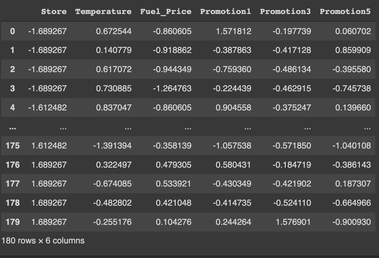
3. 제출 파일 만들기
sample_submission = pd.read_csv('./dataset/sample_submission.csv')
sample_submission['Weekly_Sales'] = predict
sample_submission.to_csv('submission.csv',index = False)
sample_submission.head()