
쇼핑몰 지점별 경진대회
요약 :
- 대회 참여를 위해 Google Colab Pro 서버를 활용하여 진행했습니다.
- 데이터 분석을 하기 위해 히스토그램, 군집화, 선형성을 확인하였습니다.
- Machine Learning Model은 scikit-learn에 있는 RandomForest모델을 활용하여 가격 예측 모델을 만들었습니다.
1. 데이터 분석
- 올바른 ML Model에 학습 시키기 위해서는 정확한 데이터 분석을 해야합니다.
- 학습(Train) 데이터, 및 테스트(Test) 데이터를 불러와 학습을 합니다. 이 때 컬럼의 갯수와 이름, 타겟 데이터 등을 파악 하여 각 변수들이 어떠한 관계가 있는지 히스토그램, 히트맵, 군집화 등 다양한 데이터 분석기법을 활용하여 분석했습니다.
- 미리 요약해드리자면 각 변수간의 선형성(linearity)을 나타내는 correlation을 파악해보면 매우 낮은 값을 갖고 있다는 것을 알 수 있었고, 따라서 예측 모델을 만들기 위해서 해당 다중선형회귀 분석 및 회귀분석에는 적합하지 않음을 확인할 수 있었습니다.
- XGBoost를 적용한 뒤 Feature의 중요도를 탐색하여 필요한 값을 선택해주었습니다.
1.1 패키지 다운로드
- 데이터 분석 및 ML 모델링에 필요한 패키지를 다운로드 합니다. 사용하는 라이브러니는 pandas, numpy 시각화를 위한 seaborn, matplotlib.pyplot ML 모델 학습을 위한 sklearn.model_selection의 train_test_split, sklearn.ensemble 의 RandomFroestRegressor, BaggingRegressor, DecisionTreeRegressor, AdaBoostRegressor, Xgboost를 이용해주었습니다.
# 데이터 분석
import pandas as pd
import numpy as np
# 데이터 분석(시각화)
import matplotlib.pyplot as plt
import seaborn as sns
# ML 모델링
from sklearn.model_selection import train_test_split
import skimage
import shap
import xgboost

# RMSE
from sklearn.metrics import mean_squared_error
.2 데이터 로드
train_data = pd.read_csv("./dataset/train.csv")
train_data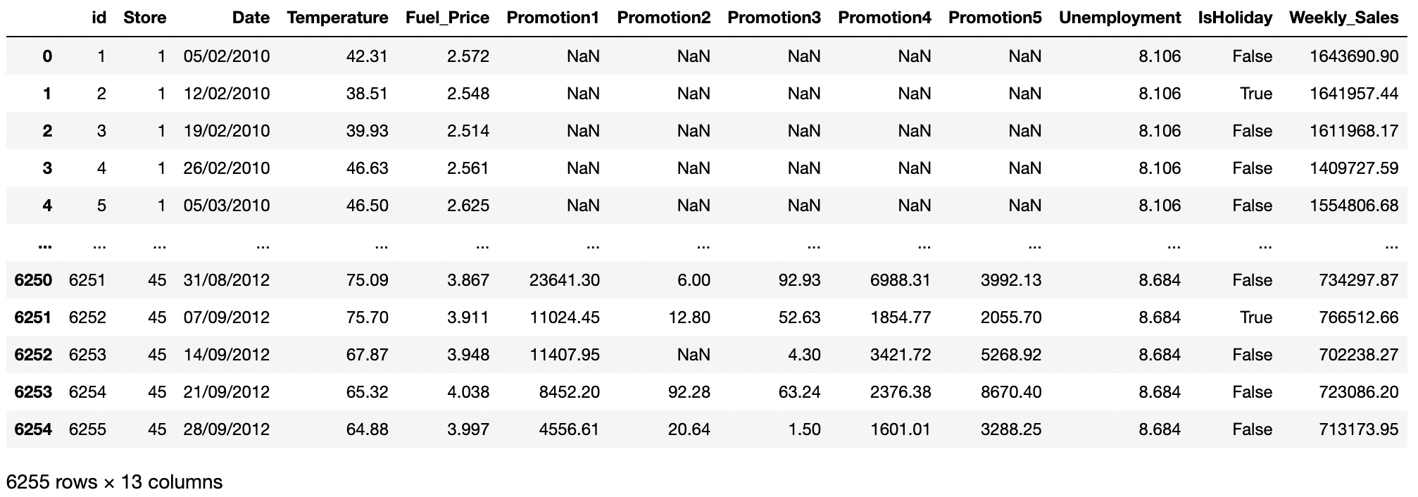
test_data = pd.read_csv("./dataset/test.csv")
test_data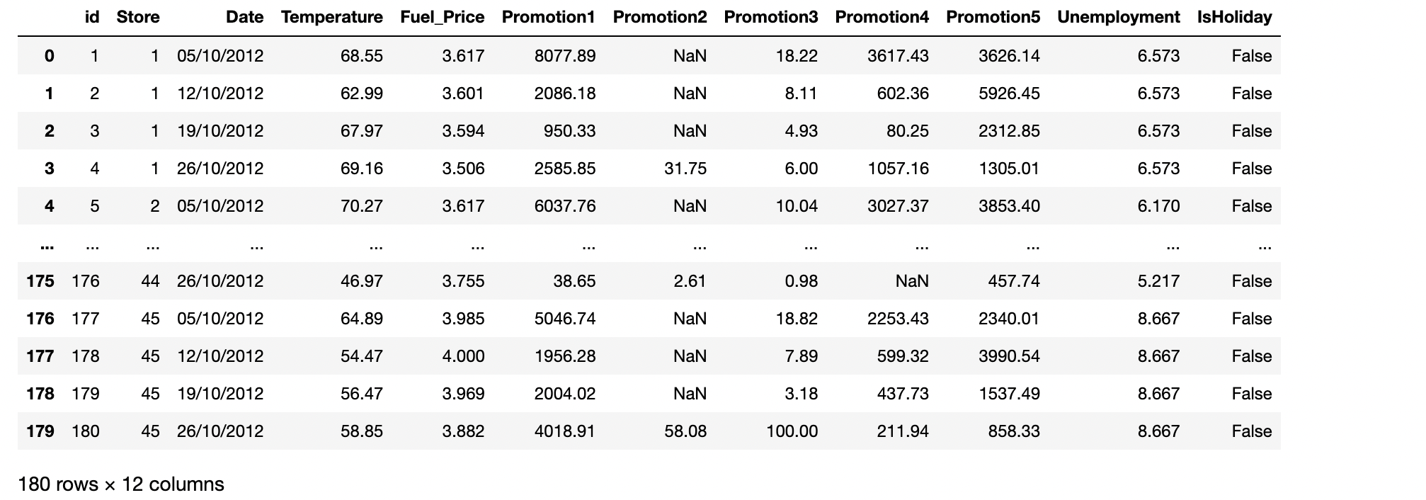
1.3 데이터 전처리
- 결측치를 제거하거나(0으로 채우거나), One-hot encoding 으로 범주형 데이터를 수치형으로 변환을 하고, 정규화를 진행합니다.
- pandas에 isna()함수와 sum()함수를 활용하여 각 컬럼에 얼마나 많은 결측치가 있는지 확인하였습니다.
# 결측치 확인
train_data.isna().sum()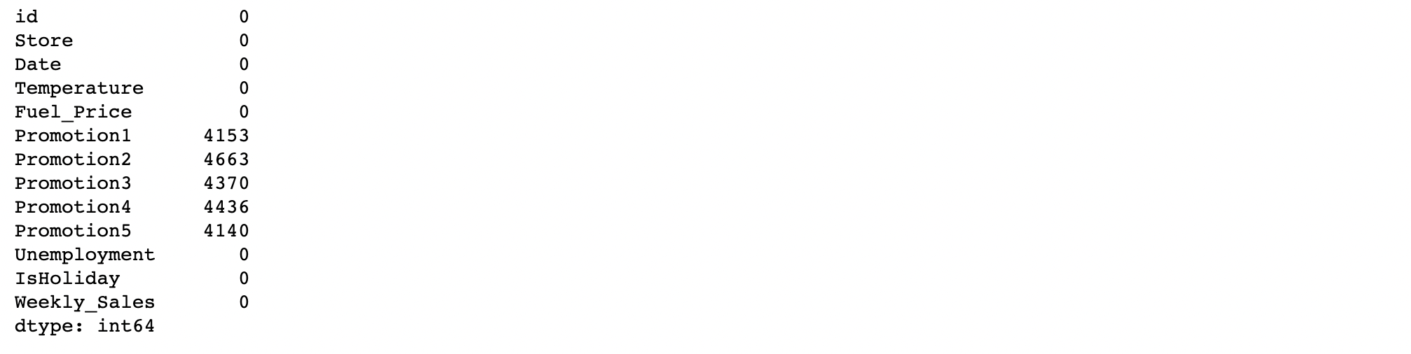
- Promotion 1~5에 Nan으로 표기된 4000개 이상입니다, 전체 데이터가 6000개정도 밖에 되지 않기 때문에 단순히 결측치를 가지고 있는 데이터를 삭제할 경우 학습데이터가 부족할 수도 있고 제대로 학습이 안될 가능성이 있기때문에 결측치는 모두 0으로 채워주도록 하겠습니다.
- 또한 Target Data인 Weekly Sales 값은 결측치가 없는 것을 알 수 있습니다.
# 결측치 0으로 채우기
train_data=train_data.fillna(0)
train_data.isna().sum()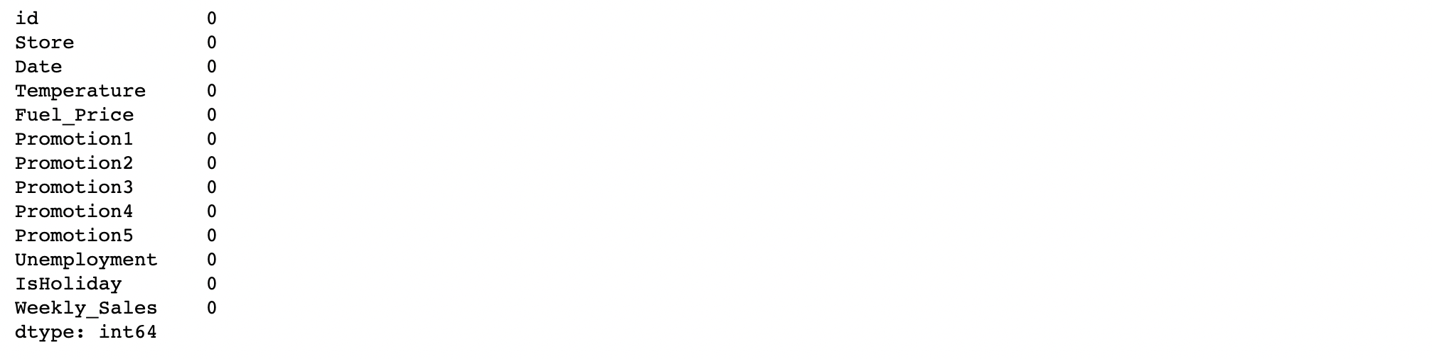
• 값이 어떤 데이터 타입의 값이 들어가 있는지 확인해줍니다.
print(train_data.columns)
print(train_data.dtypes)
print("행 열 :", train_data.shape)
• Bool 변수를 one-hot encoding을 통해서 0,1값으로 바꿔줍니다.
train_data["IsHoliday"] = train_data["IsHoliday"].astype(int)• Date데이터의 연,월,일의 값이 object형태이기 때문에 값을 바꿔줍니다.
# Date데이터의 연월일을 변환
day =[]
month=[]
year=[]
for i in range(len(train_data["Date"])):
  day.append(int(train_data.iloc[i]["Date"][0:2]))
  month.append(int(train_data.iloc[i]["Date"][3:5]))
  year.append(int(train_data.iloc[i]["Date"][6:]))
train_data["day"]=day
train_data["month"] = month
train_data["year"] = year
• pandas에 자동으로 histogram을 만들어 주는 함수인 .hist를 이용해서 histogram을 만들어줍니다.
train_data.hist(figsize=(30,20))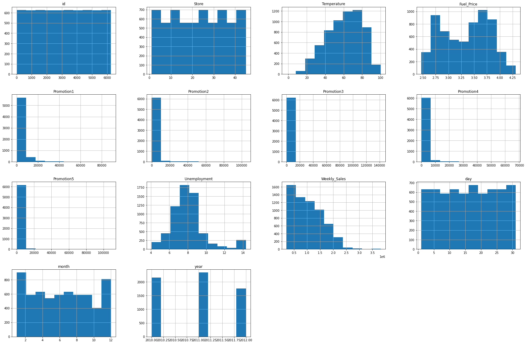
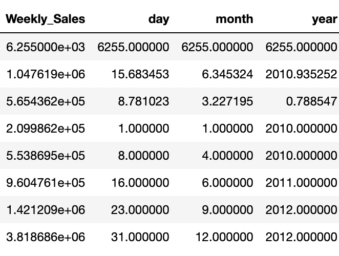
• 이제 데이터의 값의 분포를 describe함수를 통해 숫자로 확인합니다. 각 값이 mean, std, min을 살펴 분포가 어떻게 되어 있는지 파악합니다.
train_data.describe()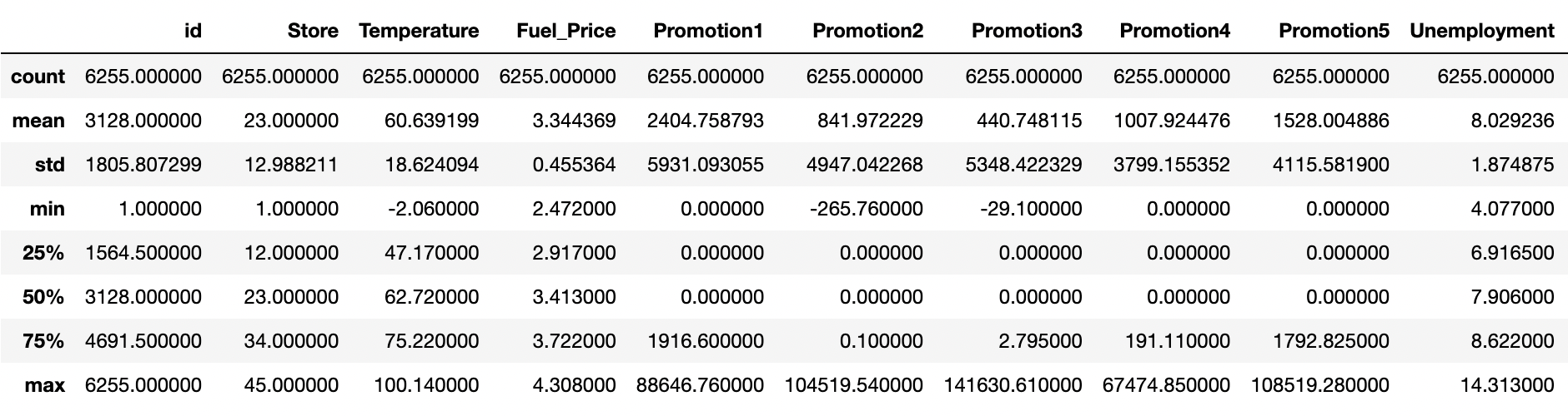
- 히스토그램과 숫자 데이터를 분석해보면 Promotion 칼럼에 해당하는 값들이 많은 값이 비워져있고 promotion1, promotion2, promotion3, promotion4, promotion5 값이 3000~5000정도이지만, 각 25%, 50% 구간이 0으로 매우 치우져있음을 알 수 있습니다. 히스토그램에서도 0에 해당하는 값들이 다른 값들보다 압도적으로 많은 것을 확인할 수 있습니다.
- 또한 Weekly_Sales의 값도 평균보다 아래의 값에 분포가 되어 있는 것을 볼 수 있습니다.
- 또한 많은 컬럼들의 숫자 범위가 크게 다른 것을 확인할 수 있습니다.
- 정규화를 적용시켜 줍니다. 정규화는 Z- 정규화를 이용할 것인데요. 데이터 분포를 통해 확인할 수 있듯이, 많은 이상치가 존재합니다. min_max를 이용할 경우 이상치에 여전히 민감하기 때문에 Z-정규화를 이용해줍니다. 분석에 활용하지 않을 id, Date 또한 Target인 Weekly_Sales를 제외한, 학습에 활용될 칼럼에 해당되는 부분을 정규화를 이용해줍니다.
# id 는 제외하고 정규화 진행
norm = train_data.drop(['id','Date', 'Weekly_Sales'],axis=1)
# z-정규화( x-평균/표준편차)
train_data_normed = (norm- norm.mean())/norm.std()
train_data_normed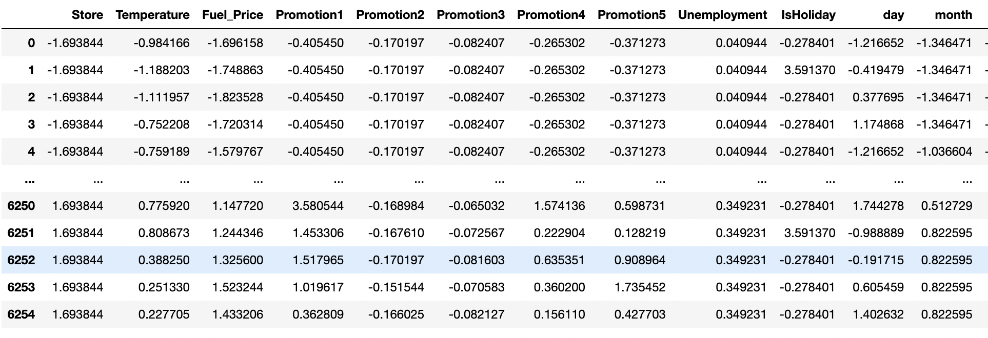
train_data_normed.hist(figsize=(30,20))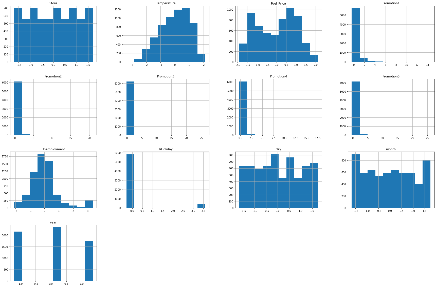
1.3 데이터 선형성(Linear Correlation)확인 - Heatmap 이용
- Target변수인 Weekly_Sales와 다른 변수와 선형성이 존재하는지 확인합니다
analysis = pd.merge(train_data_normed, train_data['Weekly_Sales'],
                left_index = True, right_index=True)
# 선형성 확인
plt.figure(figsize=(16,16))
sns.heatmap(analysis.corr(), linewidths=.5, cmap = 'Blues', annot=True)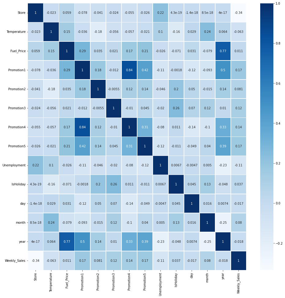
- Weekly_Sales와 다른 변수들의 correlation을 확인해보면 store정도만 0.34의 선형성을 가지고 나머지는 0.2 이하의 선형성을 가지고 있습니다. 따라서 선형성이 높지 않기 때문에 선형회귀분석이 적합하지 않는 것을 확인하였습니다.
#pairplot with Seaborn
sns.pairplot(analysis,hue='Weekly_Sales')
plt.show()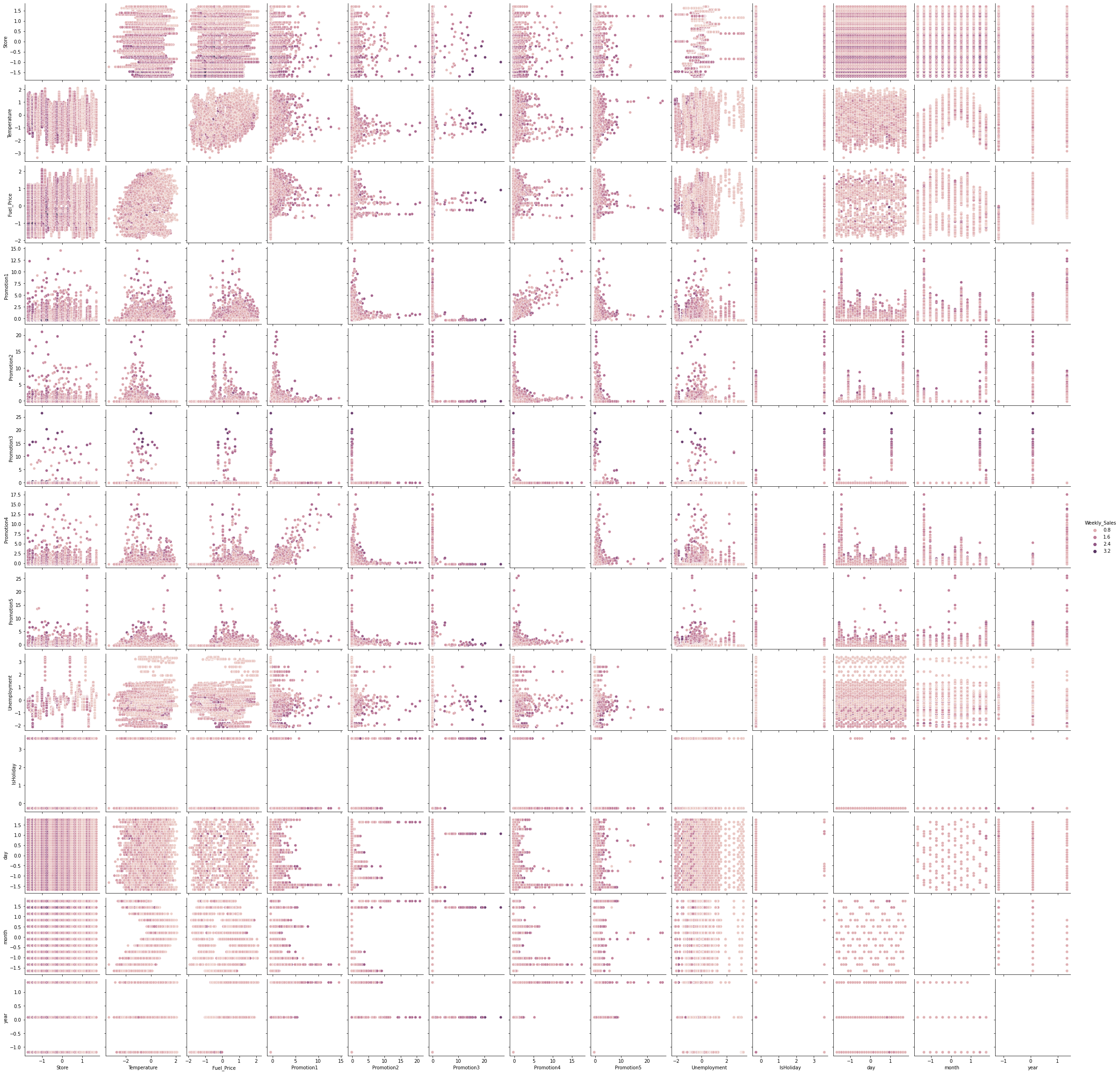
- pairplot을 확인해보면, 특정 store들을 기준으로 값이 나눠진것을 볼 수 있습니다.
- 또한 대체로 promotion값이 높을 경우 Weekly_Sales값이 높은 것을 알 수 있습니다.
- Temperature 또한 값의 분포가 나뉘는 것을 볼 수 있습니다.
2. ML 모델링
- 선형 회귀 모델, Bagging, RandomForest, Adaboost, XGBoost모델 만들기
- 종속 변수와 타겟 데이터 설정하기
2.1 데이터 학습
- 선형성이 없는 것을 확인했습니다. 다만, 실제로 모델을 만들었을때 어느정도 RMSE 값이 나오는지 체크해보았습니다.
train_y = train_data['Weekly_Sales']
train_x = train_data_normed
#drop(['IsHoliday','year'],axis=1)
#.drop(['year','Promotion1','IsHoliday','Promotion4','Promotion2','Fuel_Price'],axis=1)print(train_x.shape, train_y.shape)
2.1.1 XGboost
- Xgboost는 앙상블 기법중 Boosting 기법 중 하나로 Gradient Boosting 기법에 속합니다. Gradient Boosting 방식은 에러를 지속적으로 학습하기 때문에 과적합이 될 가능성이 높습니다. 하지만, XGBoost는 Regularization Term이 추가되어 있어 과적합을 줄여줄 수 있습니다.
Boosting이란? 앙상블 기법중 하나로오분류된 데이터에 초점을 맞추어 더 많은 가중치를 주는 방식입니다.
초기에는 모든 데이터가 동일한 가중치를 가지지만, 각 round가 종료된 후 가중치와 중요도를 계산하며, 복원 추출 시에 가중치 분포를 더 많이 고려합니다.
Boosting 기법에는 여러가지 기법이 있지만 그 중에서 Gradient Boosting 기법 중 하나인 XGboost 기법을 이용해서 모델링을 진행해주었습니다.
Gradient Boosting이란?Round의 합성 분류기의 데이터 별 오류를 예측하는 약한 분류기를 학습하는 방식으로 쉽게 말해 줄일 수 있는 오차를 학습하여 오차를 줄여나가는 방식입니다.
Feature Selection
- Feature들 중 필요하지 않은 feature을 선택하여 학습에 이용할 경우, 성능이 저하될 수 있는 문제점이 있습니다. 두번째로 Feature수가 많아져 모델이 복잡해질 경우 과적합이 될수도 잇습니다. 따라서 변수의 영향력을 파악하여 적절한 변수를 선택해야 합니다.
xgb_model= xgboost.XGBRegressor(learning_rate=0.2,
                                 n_estimators=100,
                                 max_depth=8,
                                 min_child_weight=1,
                                 gamma=0,
                                 colsample_bytree = 0.7,
                                 subsample=0.75,
                                 objective= 'reg:squarederror',
                                 nthread=-1,
                                 reg_alpha = 1e-5,
                                 scale_pos_weight=1,
                                 seed=2011)
xgb_model.fit(train_x,train_y)
predict = xgb_model.predict(train_x )
print("RMSE: {}".format((mean_squared_error(predict, train_y)**0.5)))
RMSE: 30367.758432242645
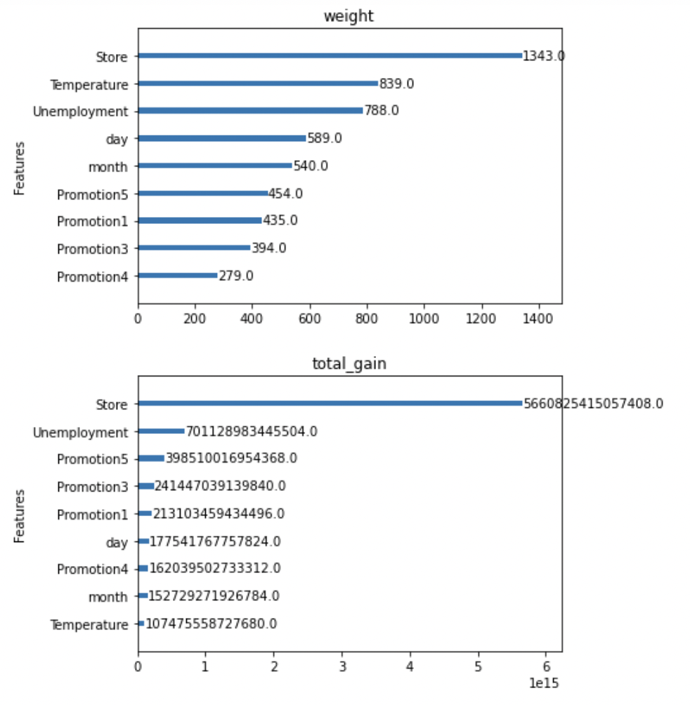
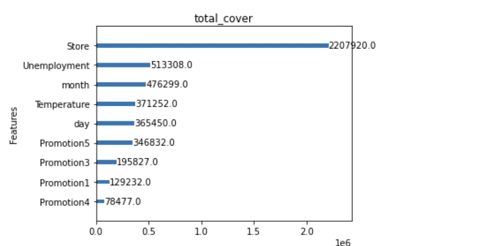
Xgboost는 변수별 중요도 파악
- Feature importance를 파악할 수 있는 함수를 제공합니다. 해당기능을 통해 어떤 변수가 영향력이 큰지 파악해보도록 합시다.
- Gain : 변수별로 손실함수를 줄여준 정도
- Weight : 데이터를 분리하는데 활용한 횟수
- Cover : Feature과 관련된 샘플의 갯수
- 단점 : 관점이 여러개라 해석이 불가능함. (consistency가 낮음)
xgboost.plot_importance(xgb_model, importance_type = 'gain', title='gain', xlabel='', grid=False)
xgboost.plot_importance(xgb_model, importance_type = 'cover', title='cover', xlabel='', grid=False)
xgboost.plot_importance(xgb_model, importance_type = 'weight', title='weight', xlabel='', grid=False)
xgboost.plot_importance(xgb_model, importance_type = 'total_gain', title='total_gain', xlabel='', grid=False)
xgboost.plot_importance(xgb_model, importance_type = 'total_cover', title='total_cover', xlabel='', grid=False)
plt.tight_layout()
plt.show()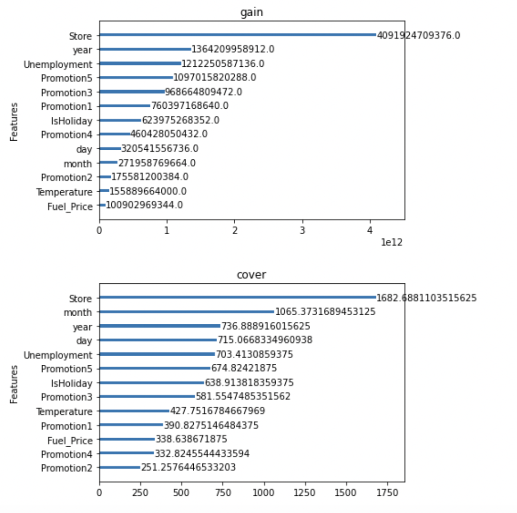
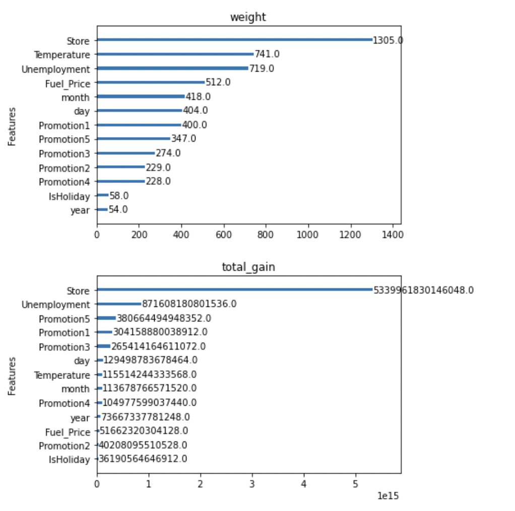
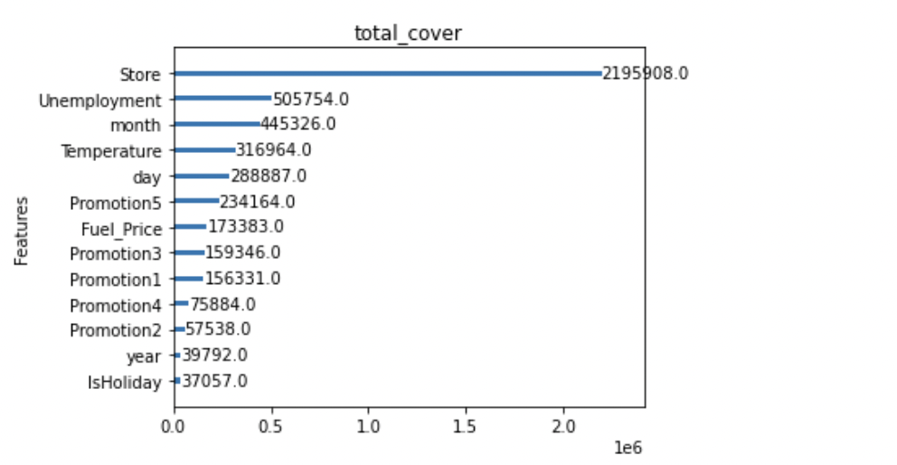
- IsHoliday와 year는 지속적으로 total_cover, total_gain, weight등에서 하위권을 형성하는 것을 알 수 있습니다.
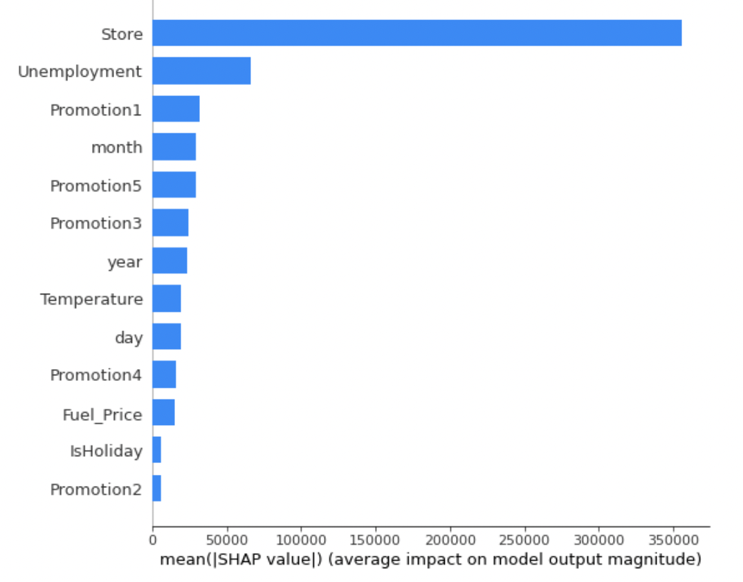
Shap Value
- Shap value 는 consistency를 보장함
- 특정 관측치 별로 중요도를 볼 수 있음
- 다양한 변수들의 조합을 통해 시각화를 할 수 있어 파악하기 쉬움
import shap
explainer = shap.TreeExplainer(xgb_model) # 트리 모델 Shap Value 계산 객체 지정
shap_values = explainer.shap_values(train_x)shap.initjs() # 자바스크립트 초기화 (그래프 초기화)
shap.force_plot(explainer.expected_value, shap_values[1,:], train_x.iloc[1,:])
# 첫 번째 검증 데이터 인스턴스에 대해 Shap Value를 적용하여 시각화
# 빨간색이 영향도가 높으며, 파란색이 영향도가 낮음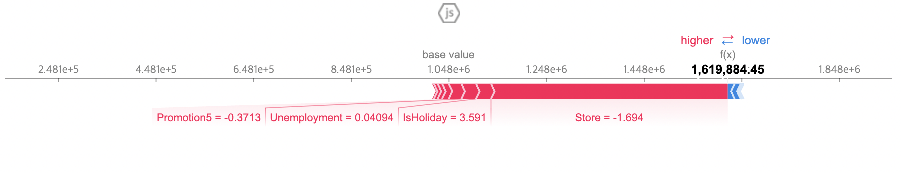
shap.summary_plot(shap_values, train_x)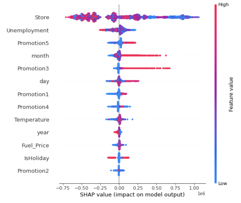
하이퍼 파라미터 튜팅
- 다음은 Xgboost는 모델을 학습시키기 위한 다양한 Parameter가 존재합니다. 해당하는 값의 문제를 해결해주기 위해 첫번째로는 정확도를 높이는 방식으로 튜닝을 진행해주고, 이후에 내용을 학습하였다
Step1. 정확도 향상
- max_depth, min_child_weight, n_estimator 하이퍼파라미터 튜닝
# 정확도 향상
from sklearn.model_selection import GridSearchCV

params = {
 'max_depth':range(3,10,3),
 'min_child_weight':range(1,6,2),
 'n_estimators':range(100,1100,100)
}
grid_xgb = GridSearchCV(estimator = xgboost.XGBRegressor(learning_rate=0.1,
                                                         n_estimators=1000,
                                                         max_depth=5,
                                                         min_child_weight=1,
                                                         gamma=0,
                                                         subsample=0.8,
                                                         colsample_bytree=0.8,
                                                         objective= 'reg:squarederror',
                                                         nthread=-1,
                                                         scale_pos_weight=1,
                                                         seed=2019),
                        param_grid = params, n_jobs=-1, cv=10)
grid_xgb.fit(train_x,train_y)
predict=grid_xgb.predict(train_x)
print("RMSE:",mean_squared_error(train_y, predict)**0.5)
print(grid_xgb.best_params_)
Step2
- gamma 하이퍼파라미터 튜닝
from sklearn.model_selection import GridSearchCV

params = {
    'gamma':[i/10.0 for i in range(0,5)]
}
grid_xgb = GridSearchCV(estimator = xgboost.XGBRegressor(learning_rate=0.1,
                                                         n_estimators=100,
                                                         max_depth=3,
                                                         min_child_weight=3,
                                                         gamma=0,
                                                         subsample=0.8,
                                                         colsample_bytree=0.8,
                                                         objective= 'reg:squarederror',
                                                         nthread=-1,
                                                         scale_pos_weight=1,
                                                         seed=2019),
                        param_grid = params, n_jobs=-1, cv=10)
grid_xgb.fit(train_x,train_y)
predict=grid_xgb.predict(train_x)
print("RMSE:",mean_squared_error(train_y, predict)**0.5)
print(grid_xgb.best_params_)
Step3
- colsample_bytree, subsample 하이퍼파라미터 튜닝
from sklearn.model_selection import GridSearchCV

params = {
    'colsample_bytree':[i/10.0 for i in range(6,10)],
    'subsample':[i/100.0 for i in range(40,80)],

}
grid_xgb = GridSearchCV(estimator = xgboost.XGBRegressor(learning_rate=0.1,
                                                         n_estimators=100,
                                                         max_depth=3,
                                                         min_child_weight=3,
                                                         gamma=0,
                                                         subsample=0.6,
                                                         colsample_bytree=0.74,
                                                         objective= 'reg:squarederror',
                                                         nthread=-1,
                                                         scale_pos_weight=1,
                                                         seed=2019),
                        param_grid = params, n_jobs=-1, cv=10)
grid_xgb.fit(train_x,train_y)
predict=grid_xgb.predict(train_x)
print("RMSE:",mean_squared_error(train_y, predict)**0.5)
print(grid_xgb.best_params_)
from sklearn.model_selection import GridSearchCV

params = {
    'subsample':[i/100.0 for i in range(40,80)],
}
grid_xgb = GridSearchCV(estimator = xgboost.XGBRegressor(learning_rate=0.1,
                                                         n_estimators=100,
                                                         max_depth=3,
                                                         min_child_weight=3,
                                                         gamma=0,
                                                         colsample_bytree = 0.6,
                                                         subsample=0.74,
                                                         objective= 'reg:squarederror',
                                                         nthread=-1,
                                                         scale_pos_weight=1,
                                                         seed=2019),
                        param_grid = params,n_jobs=-1, cv=10)
grid_xgb.fit(train_x,train_y)
predict=grid_xgb.predict(train_x)
print("RMSE:",mean_squared_error(train_y, predict)**0.5)
print(grid_xgb.best_params_)
Step 4.
- Regularization Parameter 튜닝
from sklearn.model_selection import GridSearchCV

params = {

    'reg_alpha':[1e-5, 1e-2, 0.1, 1, 100]
}
grid_xgb = GridSearchCV(estimator = xgboost.XGBRegressor(learning_rate=0.1,
                                                         n_estimators=100,
                                                         max_depth=3,
                                                         min_child_weight=3,
                                                         gamma=0,
                                                         colsample_bytree = 0.6,
                                                         subsample=0.74,
                                                         objective= 'reg:squarederror',
                                                         nthread=-1,
                                                         scale_pos_weight=1,
                                                         seed=2019),
                        param_grid = params,n_jobs=-1, cv=10)
grid_xgb.fit(train_x,train_y)
predict=grid_xgb.predict(train_x)
print("RMSE:",mean_squared_error(train_y, predict)**0.5)
print(grid_xgb.best_params_, grid_xgb.best_score_)
Learning Rate
- learning_rate 하이퍼 파라미터 튜닝
params = {
    'learning_rate':[0.001, 0.1, 0.2, 0.3, 0.4, 0.5, 0.6, 0.7, 0.8, 0.9]
}
grid_xgb = GridSearchCV(estimator = xgboost.XGBRegressor(learning_rate=0.1,
                                                         n_estimators=100,
                                                         max_depth=3,
                                                         min_child_weight=3,
                                                         gamma=0,
                                                         colsample_bytree = 0.6,
                                                         subsample=0.74,
                                                         objective= 'reg:squarederror',
                                                         nthread=-1,
                                                         scale_pos_weight=1,
                                                         reg_alpha = 100,
                                                         seed=2019),
                        param_grid = params,n_jobs=-1, cv=10)
grid_xgb.fit(train_x,train_y)
predict=grid_xgb.predict(train_x)
print("RMSE:",mean_squared_error(train_y, predict)**0.5)
print(grid_xgb.best_params_, grid_xgb.best_score_)
최종 XGboost Regressor에 체크
import tqdm
best_seed = []
for i in tqdm.notebook.tqdm(range(2019)):
	xgb_model=xgboost.XGBRegressor(learning_rate=0.1,
	n_estimators=100,
	max_depth=3,
	min_child_weight=3,
	gamma=0,
	subsample=0.6,
	colsample_bytree=0.74,
	objective= 'reg:squarederror',
	nthread=-1,
	scale_pos_weight=1,
	reg_alpha = 100,
	seed=i)
	xgb_model.fit(train_x,train_y)
	predict=xgb_model.predict(train_x)
	best_seed.append(((mean_squared_error(predict, train_y)**0.5),i))
best_seed.sort()
print(best_seed[0])
xgboost.plot_importance(xgb_model, importance_type = 'gain', title='gain', xlabel='', grid=False)
xgboost.plot_importance(xgb_model, importance_type = 'cover', title='cover', xlabel='', grid=False)
xgboost.plot_importance(xgb_model, importance_type = 'weight', title='weight', xlabel='', grid=False)
xgboost.plot_importance(xgb_model, importance_type = 'total_gain', title='total_gain', xlabel='', grid=False)
xgboost.plot_importance(xgb_model, importance_type = 'total_cover', title='total_cover', xlabel='', grid=False)
plt.tight_layout()
plt.show()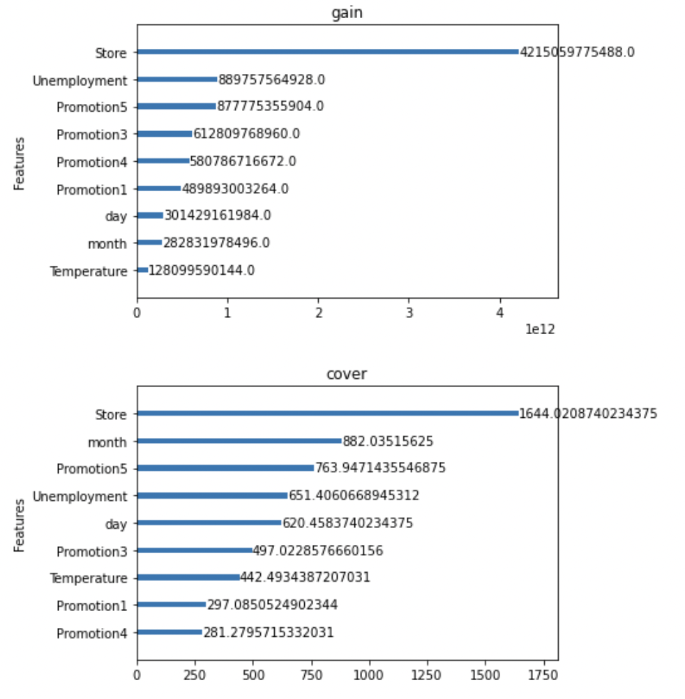
2.2 최종 Test Data 체크 및 Submission Data 생성
#전처리
test_data["IsHoliday"] = test_data["IsHoliday"].astype(int)
test_data=test_data.fillna(0)
# Date데이터의 연월일을 변환
day =[]
month=[]
year=[]
for i in range(len(test_data["Date"])):
  day.append(int(test_data.iloc[i]["Date"][0:2]))
  month.append(int(test_data.iloc[i]["Date"][3:5]))
  year.append(int(test_data.iloc[i]["Date"][6:]))
test_data["day"]=day
test_data["month"] = month
test_data["year"] = year
# 필요없는 데이터 제외하고
normed = test_data.drop(['id','Date','year', 'Fuel_Price', 'IsHoliday','Promotion2'],axis=1)
#drop(['id','Date','year','Promotion1','IsHoliday','Promotion4','Promotion2'],axis=1)
# z-정규화
test_data_normed = (normed- normed.mean())/normed.std()
test_data_normed=test_data_normed.fillna(0)
test_data_normed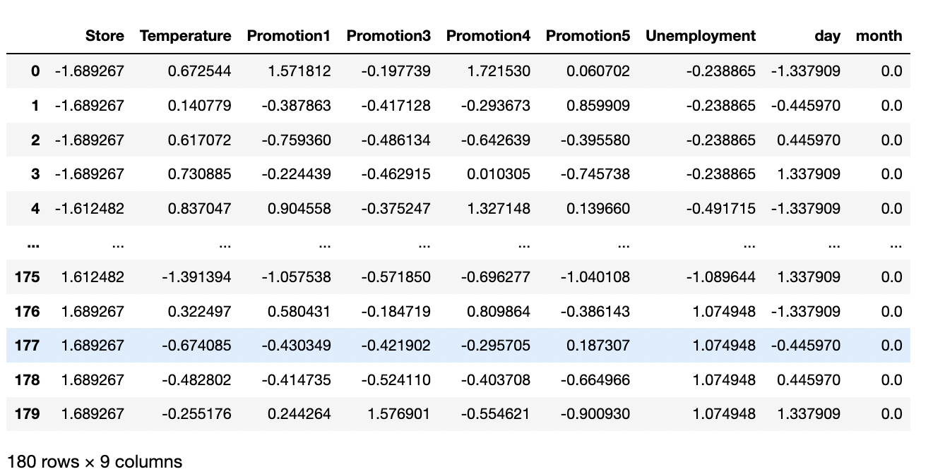
predict = xgb_model.predict(test_data_normed)3. 제출 파일 만들기
sample_submission = pd.read_csv('./dataset/sample_submission.csv')
sample_submission['Weekly_Sales'] = predict
sample_submission.to_csv('submission.csv',index = False)
sample_submission.head()
후기
위와 같은 코드로 30번 정도 제출하여, Public Score 151등으로 마무리 했다. 아쉬운 등수인데, 마지막 제출정도 코드상의 문제점을 파악할 수 있었다. 바로 Train Set에서는 총 여러해의 정보가 활용되었는데, Test Set에서는 랜덤하게 나누어져있지않고 특정 해의 특정 월정보가 적혀있었다. 따라서 정규화를 진행하면 해당 부분에 대한 데이터가 없어지는 오류가 있었는데, 테스트 데이터에 대한 분석을 아예 진행하지 않고 진행해서 해당 부분에 대한 오류가 발생한 것 같았다. 물론 테스트 데이터를 모델에 활용하면 안되겠지만, 적어도 분포가 Test와 Train Data가 다른지 아닌지정도는 파악해야될 것 같다는 생각이 들었다. Public Score는 151등, Private Score는 172등 정도로 전체 700팀 정도에서 상위 25%안에 드는 성적을 거둘 수 있었던 것 같다.
- Public Score

- Private Score