Fully Convolutional Networks for Semantic Segmentation

Paper: Fully Convolutional Netowrks for Semantic Segmentation

0. Abstract

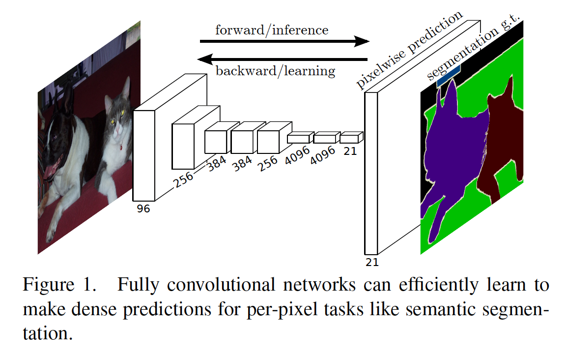
Fully Convolutional network (FC layer가 없는)을 활용하여 input 이미지의 크기에 상관 없이 segmentation 결과물을 효과적으로 얻을 수 있다.

현대의 classification에 사용되는 네트워크 (AlexNet, VGGnet, GoogLeNet)을 FCN으로 변형하고 fine-tuning을 통해 segmentation task들을 수행할 수 있다.

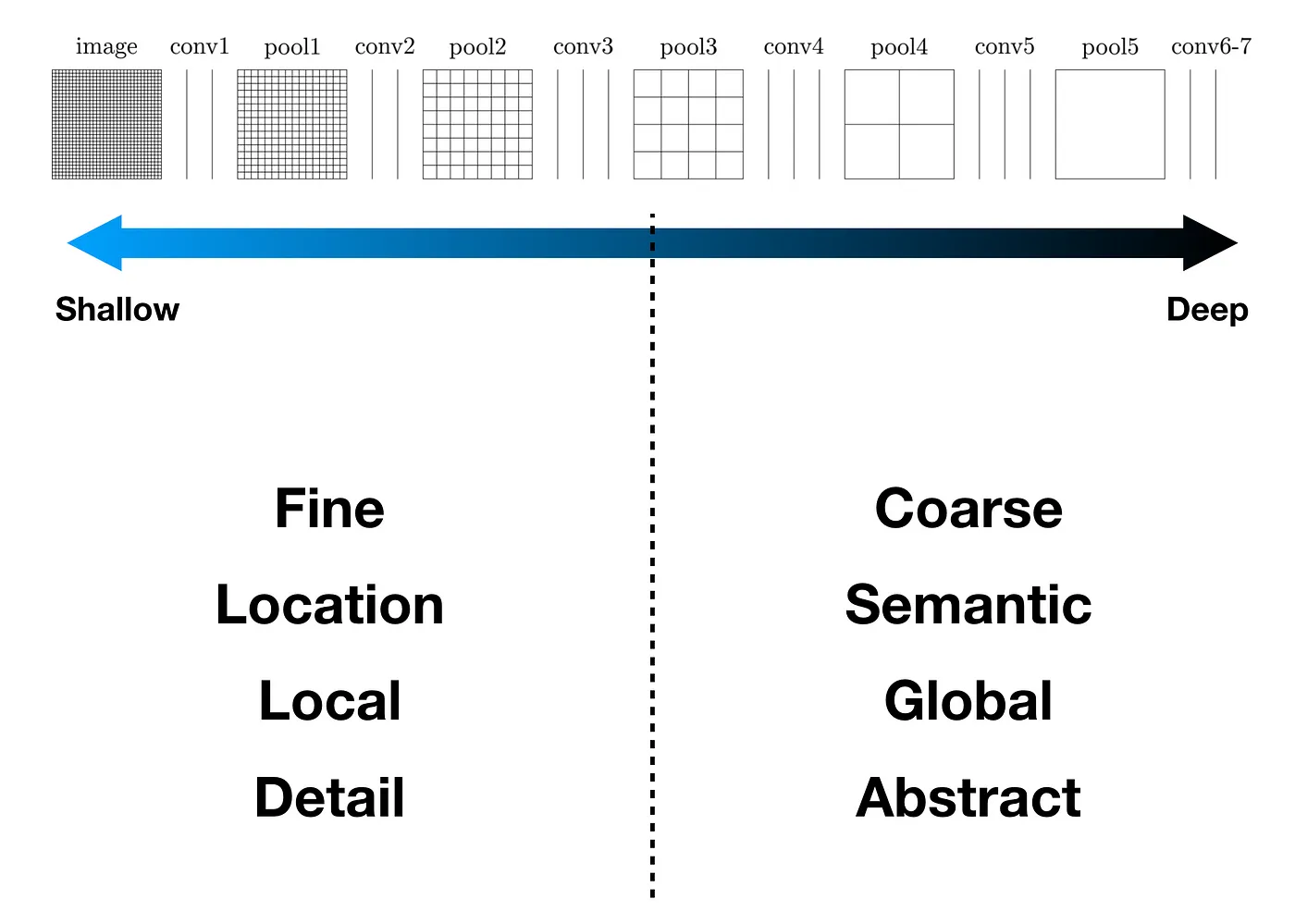
deep, coarse layer에서 보여주는 semantic 정보와 shallow, fine layer에서 나타나는 appearance 정보를 결합해 보다 정확하고 세부적으로 segmentation 과정을 수행한다.

1. Introduction

Convolutional network들은 classification, object detection task에 대해서 뛰어난 성능을 보여주었다. 그 다음 과정으로는 자연스럽게, 이미지 안의 pixel단위의 분석으로 넘어가게 된다.(Semantic Segmentation)

이 논문에서는, fully convolutional network (FCN)을 end-to-end, pixels-to-pixels 방식으로 학습시켜 기존 SOTA를 뛰어넘었다. 최초로 (1) pixelwise prediction, (2) supervised pre-training 방식을 사용한다. 또한, FCN을 이용하여 input의 사이즈에 제한이 없다. 학습과 추론 과정에서 모두 전체 이미지를 모두 사용하는 방식(whole-image-at-a-time)을 사용한다.

이전의 연구에서는 patchwise 방식을 사용했지만, 이 방식은 모델을 효율적으로 학습시킬 수 없고, 전체 이미지를 사용했을때와 결과가 비슷하게 나오기 때문에 이 모델에서는 사용하지 않았다.

Patch: 하나의 이미지에서 object은 그대로 두고 background를 제거한 것이다.

Patchwise training이란? 하나의 이미지를 subimage로 잘라 각각을 training에 이용하는 방식이다. 하지만, 이 방식은 같은 이미지 안에서 중복되게 update하게 되는 부분이 많이 생기게 되어 computation이 더 많아진다. 또한, 각각의 receptive field가 같다면, training 결과도 같게 된다. (https://stats.stackexchange.com/questions/266075/what-is-the-difference-between-patch-wise-training-and-fully-convolutional-train)

Segmentation task에는 크게 semantic 정보와 location 정보를 얻는 것이 중요하다. global information을 이용해 주로 물체가 무엇인지 파악하고, local information을 통해 물체가 어디에 있는지 파악할 수 있다. 이 논문에서는 skip architecture을 고안해 deep, coarse, semantic 정보와 shallow, fine, appearance 정보를 통합한 결과물을 얻을 수 있다.

2. Related Work

Fully Convolutional networks

• Matan et al - convnet에서 arbitrary-sized input
• Sermanet et al - Sliding window detection
• Pinherio and Collobert - semantic segmentation
• Eigen et al - image restoration
• Tompson et al - Fully convolutional training
• He et al - classification net에서 feature extractor을 만들기 위해 non-convolutional 부분을 무시함.

Dense prediction with convnets

Semantic Segmentation task는 이미지에 있는 모든 픽셀에 대해 예측하기 때문에 dense prediction이라고 부른다.

위의 논문들과 더불어, 다음과 같이 여러가지 접근방식들이 소개되어 있다:

• small models restricting capacity and receptive fields
• patchwise training
• post-processing by superpixel projection, random field regularization, filtering, or local classification
• input shifting and output interlacing for dense output as introduced by OverFeat
• multi-scale pyramid processing
• saturating tanh nonlinearities
• ensembles

위에서 소개한 방식들을 사용하지 않고, 이 논문에서는 image classification을 superviesd pre-training으로 사용하고, 이미지 전체에 대한 input과 ground truth를 활용해 fully convolutional network를 fine-tuning한다.

3. Fully Convolutional Network

convnet의 각 layer에서 데이터는 3차원 array로 이루어져 있다. $h \times w \times d$

• h, w: 2차원 공간의 크기
• d: channel의 갯수
  -> 첫번째 Layer은 크기 $h \times w$, color channel d인 image가 된다.

또한, 한 layer의 feature map과 kernel의 convolution 연산을 통해 다음 layer의 feature map을 얻을 수 있는데, 상위 layer의 feature 값을 얻을 때의 연산에 필요한 이전 layer feature의 범위를 receptive field라고 부른다.

Convnet은 기본적으로 평행이동에 영향을 받지 않는다.(translation invariance)

또한, deconvolution layer을 사용해 coarse output map을 얻을 수 있다.

3.1 Adapting classifiers for dense prediction

일반적인 ConvNet들은 다음과 같이 convolution layer들 이후에 fully connected layers (FC layers)를 거쳐 output을 얻는다.

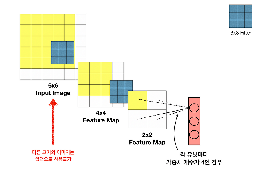
이때, FC layer들은 고정된 크기의 input을 받아야 하기 때문에, input으로 사용할 수 있는 이미지의 크기가 정해져 있다. 또한, FC layer로 변형하게 되면 공간적인 정보를 잃어버리게 된다.

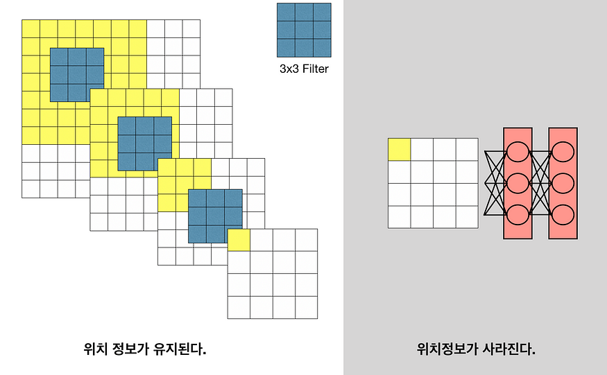
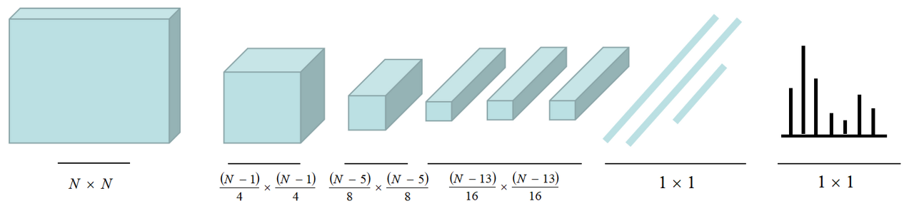
그래서 FC layer부분을 1x1 convolutional layer로 바꾸어 주어 공간 정보도 보존하고, arbitrary-sized input을 사용할 수 있게 해준다.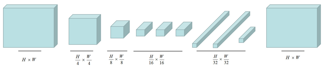

또한 다음과 같이 FCN을 구성하면 기존의 ConvNet들보다 훨씬 빠른 연산이 가능하다.

3.2 Shift-and-stitch is filter rarefaction

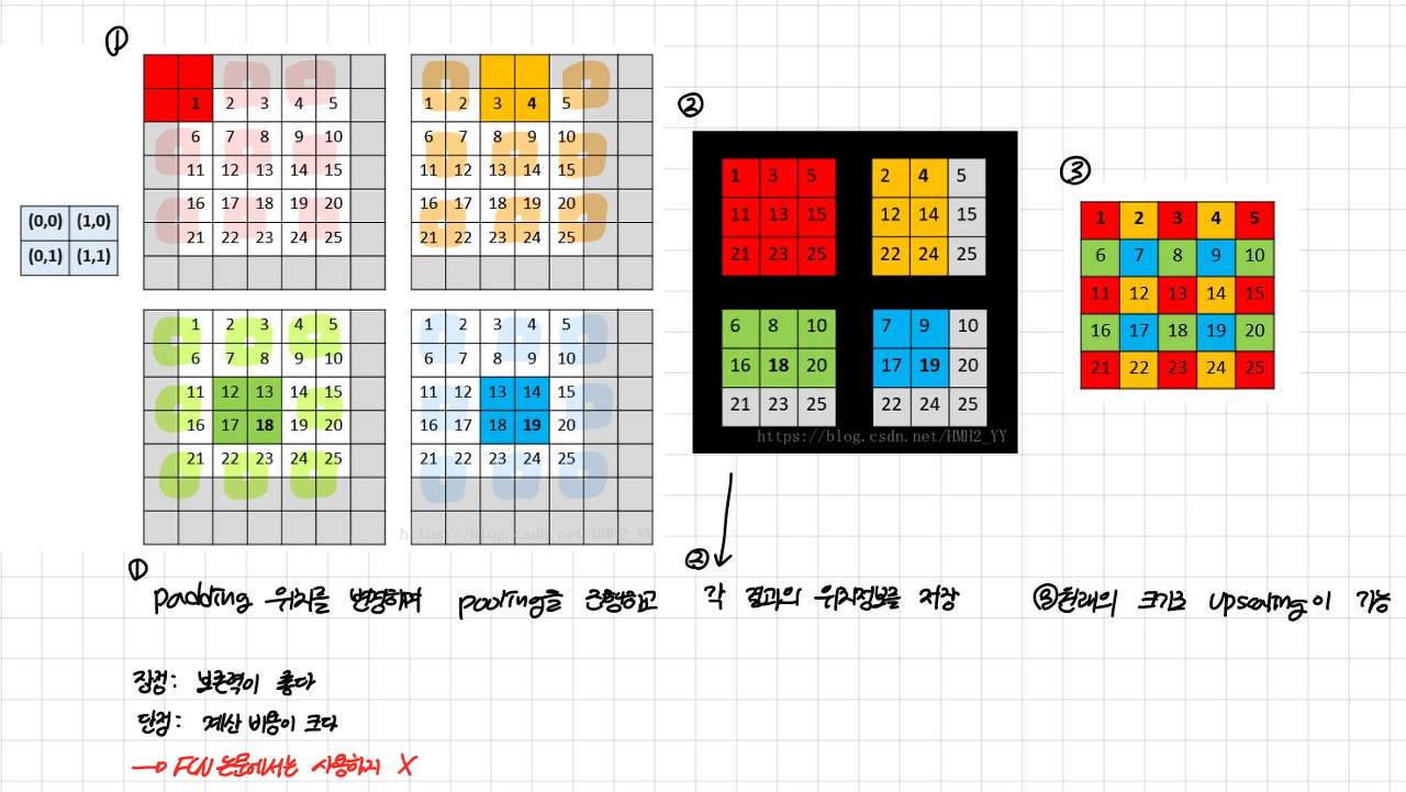
Shift-and-stitch방식: 하나의 이미지에 대해서 위아래와 좌우의 padding값을 각각 다르게 설정한 뒤 각각에 대해 pooling을 진행한다. 그러면 결과값들을 이용해 다시 upsampling이 다음과 같이 가능해진다:

논문에서는 upsampling 과정에서 기존의 Shift-and-stitch 방식을 사용하지 않는다. 대신에, 다음과 같이 shift-and-stitch과 유사한 효과를 낼 수 있는 trick을 소개한다:

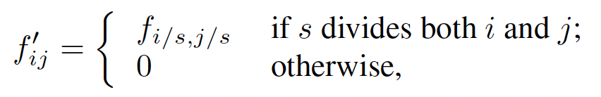
• $i, j$: output shape
• $s$: stride
  -> stride로 나누어 떨어지는 값은 기존의 값으로 설정하고, 나머지는 0으로 채워준다.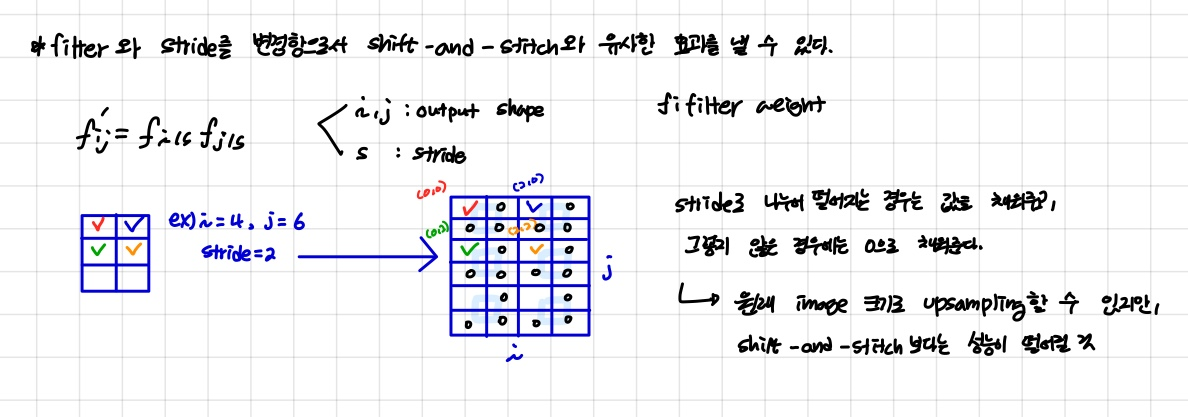

3.3 Upsampling is backwards strided convolution

coarse output를 dense pixel로 변환하는 기법으로 interpolation이 있다. 예시로, 가까운 pixel들의 값을 거리에 반비례하게 참고해 값을 설정하는 bilinear interpolation 방식이 있다.

이 논문에서는 학습이 가능한 backwards convolution (deconvolution)을 사용한다.

convolution 연산의 반대로 진행하며, convolution과 같이 weight filter가 있어 end-to-end 학습이 가능하다.

3.4 Patchwise training is loss sampling

이 논문에서는 앞에서 설명한 patchwise training을 사용하지 않는다. patchwise training은 class imbalance 문제를 해결할 수 있지만, patch간의 위치 정보를 잃게 된다. 또한, 전체 이미지를 학습할 때와 결과가 동일하며, 계산적으로도 전체 이미지를 학습하는 것이 더 유리하다고 한다. class imbalance 문제는 loss에 가중치를 다르게 부여하여 해결할 수 있다.

"Whole image training is effective and efficient"

4. Segmentation Architecture

먼저 Classifier을 FCN으로 변환한 후, segmentation으로 fine-tuning과정을 거친다. 그 후, skip architecture를 추가하여 coarse, semantic정보와 local, appearance정보를 합쳐준다.

4.1 From classifier to dense FCN

논문에서는 Base Network로 AlexNet, VGG16, GoogLeNet 세가지를 사용하였다. 마지막 FC Layer 대신에 1x1x21 convolution layer로 대체하고, (channel의 수가 21인 이유는 사용한 PASCAL VOC 2011의 class 수가 21개이다.) 이어서 deconvolution layer을 이용하여 coarse map을 pixel-dense output로 upsample해준다.

또한, 기존의 Classifier에 Segmentation으로 fine-tuning 해주는 작업을 통해 의미있는 퍼포먼스 향상이 있었다. (가장 안좋은 모델도 SOTA의 75% 성능을 보여줌)

4.2 Combining what and where

4.1에서 구성한 네트워크는 뛰어난 성능을 보여주지만, 결과물을 보면 디테일한 부분이 표현되지 않는다.(FCN-32s)

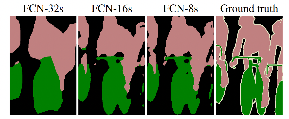
이를 해결하기 위해, 앞에서 언급한 skip architecture를 사용한다. base network의 최종 단계까지 가기 이전의 feature map들을 추가로 이용하여 단계적으로 upsampling을 진행한다.

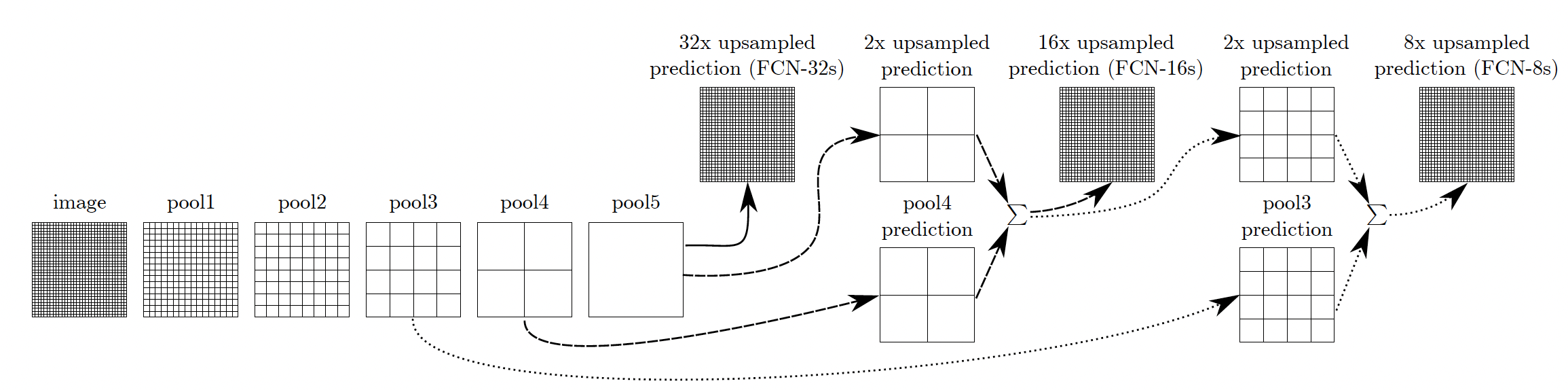
• FCN-32s: pool5에서 x32 upsampling
• FCN-16s: pool5에서 x2 upsampling한 값과 pool4를 합친 뒤 x16 upsampling
• FCN-8s: 위의 단계에서 x2 upsampling한 값과 pool3을 합친 뒤 x8 upsampling

skip architecture의 효과가 나타나는 것을 다음의 표와 위의 그림을 통해 볼 수 있다: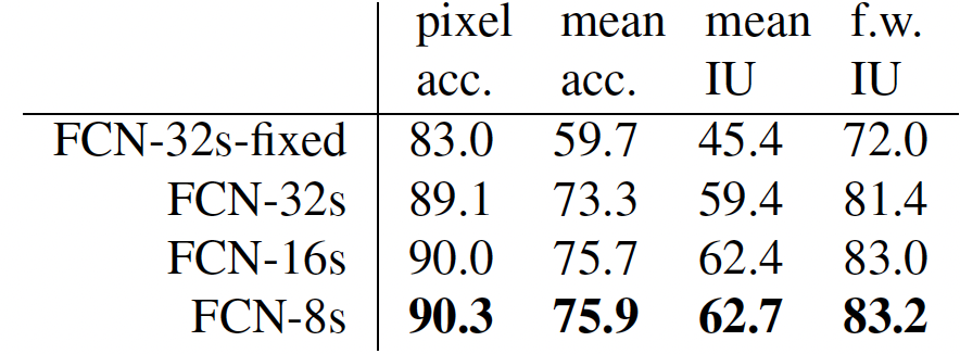

4.3 Experimental framework

Patch Sampling

전체 이미지를 이용해 학습하는 것과 patch로 나누어 학습하는 것에 차이가 없으며, 전체 이미지를 이용해 학습했을 때 더 빠르게 converge하다는 것을 아래의 그래프를 통해서 알 수 있다: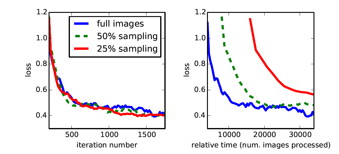

Class Balancing

각 class마다 loss의 가중치를 다르게 부여해 class imbalance 문제를 보완한다.

Dense Prediction

deconvolutional filter와 bilinear interpolation을 이용해 upsampling 과정을 진행한다.

5. Result

Semantic Segmentation과 Scene parsing Dataset인 PASCAL VOC, NYUDv2, SIFT Flow에 대해서 테스트 완료.

Semantic Segmentation: 각각의 픽셀에 대해서 알려진 객체에 한해 class를 분류하는 작업
Scene parsing: 이미지 내의 모든 픽셀에 대하여 categorize하는 작업

Metric

$n_{ij}$: class $i$에 속하는 pixel 중에서 class $j$라고 예측한 pixel의 수
$t_i = \sum_j n_{ij}$(class $i$의 총 픽셀 수) 라고 할때, 다음과 같이 네가지 지표로 평가한다:

• pixel accuracy: $\cfrac{\sum_i n_{ii}}{\sum_i t_i}$
• mean accuracy: $\cfrac{1}{n_{cl}}\sum_i \cfrac{n_{ii}}{t_i}$
• mean IoU: $\cfrac{1}{n_{cl}}\cdot\cfrac{\sum_in_{ii}}{(t_i + \sum_j n_{ji} - n_{ii})}$
• frequency weighted IoU: $\cfrac{1}{\sum_kt_k}\cdot\cfrac{\sum_it_in_{ii}}{(t_i + \sum_j n_{ji} - n_{ii})}$

---

Reference

https://asidefine.tistory.com/165

https://medium.com/@msmapark2/fcn-논문-리뷰-fully-convolutional-networks-for-semantic-segmentation-81f016d76204

---