DEtection TRansformer

Paper: End-to-End Object Detection with Transformers

이번에 리뷰할 논문은 DETR (Detection Transformer) 입니다. DETR은 Semantic Segmentation이 아닌, Object Detection를 주요 task로 다루지만, CNN과 Transformer구조를 함께 사용하며 Panoptic Segmentation (Semantic + Instance Segmentation)에서도 뛰어난 성능을 보여주기 때문에, 간단하게 살펴봅시다.

0. Abstract

Object Detection에서 주로 사용하는 후처리 방식인 non-maximum suppression (NMS)이나 anchor generation 방식을 사용하지 않고 bipartite matching을 이용한 set prediction과 Transformer encoder-decoder 구조를 사용해 직접 output box set을 얻어내는 구조를 사용합니다.

1. Introduction

Object Detection은 bounding box와 해당 box 안의 class label을 예측하는 task 입니다. 많은 이전의 모델들은 여러개의 proposal, anchor, window center을 얻은 다음에 NMS 등의 중복 제거 방식을 사용해 최종 결과물을 얻습니다.

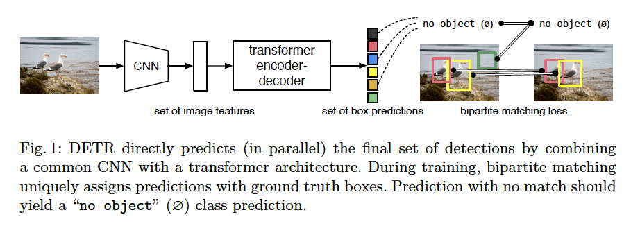
이 논문에서는 위의 그림과 같이 CNN과 Transformer encoder-decoder을 사용해 직접 최종 output을 얻을 수 있습니다. set loss function을 이용하여 gt와 예측값 사이에 bipartite matching을 이용해 end-to-end 학습이 가능합니다. 또한, transformer을 이용해 permutation-invariant한 연산이 가능해 parallel하게 처리할 수 있습니다. (Transformer은 set 연산)

2. Related Works

2.1 Set Prediction

set을 직접적으로 예측하는 모델은 이전에는 없고, NMS등을 활용해서 후처리를 해주는 방식으로 접근한다. 이번 모델은 Hungarian algorithm을 이용해서 gt와 예측값 사이의 bipartite matching을 이용해 loss값을 설정해 직접적으로 학습한다.

2.2 Transformers and Parallel Decoding

NLP에서 주로 활용되던 RNN에서 Transformer로 대부분 대체하고 있고, CV등의 다양한 도메인에까지 활용되고 있습니다.

2.3 Object Detection

기존의 2-stage Detector, 1-stage Detector의 경우 주로 학습 이전에 가정을 통해 proposal에 대한 정보를 미리 설정하고 진행한 후 (고정된 크기의 anchor들을 사용하거나, box center을 고정) 후처리를 통해 결과물을 가공합니다.

3. The DETR model

(1) gt box와 예측된 box의 set 사이의 loss를 설정해주고, (2) 이미지를 input으로 받아 object set를 반환하는 구조를 이용해야 direct set prediction이 가능합니다.

3.1 Object detection set prediction loss

DETR은 N개의 prediction을 가진 set를 output으로 합니다. (N은 실제 이미지 안의 object보다 꽤 큰 값) 이때, ground truth와 bipartite matching을 했을 때 가장 작은 값을 다음의 수식으로 나타낼 수 있습니다:

• $y$: ground truth, $\hat{y} = [\hat{y}_i]_{i=1}^N$: N개의 prediction
• $y$는 $\varnothing$으로 패딩되어 길이 N

$\mathcal{L}_{match}(y_i, \hat{y}_{\sigma(i)})$: $y_i$와 $\hat{y}_{\sigma(i)}$ 사이의 matching cost. 이때 Hungarian algorithm을 이용하여 빠르게 계산할 수 있다. class prediction과 box prediction에 대한 cost 모두 담고 있으며, 수식으로 나타내면 다음과 같다:

• $y_i = (c_i, b_i)$
• $c_i$: class label ($\varnothing$ 포함)
• $b_i \in [0,1]^4$: box center 좌표 (2d), heignt, width
• $\hat{p}_{\sigma(i)}(c_i)$: index $\sigma(i)$이 class $c_i$로 예측할 확률

위의 matching cost가 가장 적은 set를 구한 뒤에, Hungarian loss를 다음과 같이 설정해 모델을 학습시킨다.

• $\hat{\sigma}$: 맨 첫번째 수식 (set matching cost)의 값이 가장 작은 set.
• $c_i = \varnothing$인 경우 log weight를 10배 줄인다.

Bounding Box loss

3.2 DETR architecture

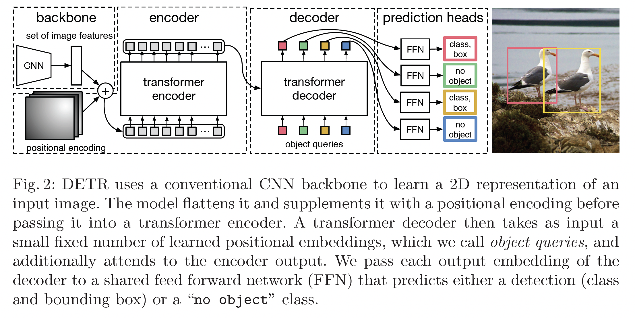
Backbone

• input image: $x_{img} \in \mathbb{R}^{3 \times H_0 \times W_0}$
• CNN output figure: $f \in \mathbb{R}^{C \times H \times W}$, C = 2048, H, W = $\frac{H_0}{32}, \frac{W_0}{32}$

Transformer Encoder

• 먼저, 1x1 conv 를 거쳐 $z_0 \in \mathbb{R}^{d \times H \times W}로 변환$
• $z_0$을 1d (length: $d \times HW$)로 변환 후 positional encoding을 추가한다.

Transformer Decoder

• N개의 object query를 설정해(learnable) N개의 prediction을 output으로 갖는다.

  object query 개념이 잘 이해가 되지 않아 참고할만한 링크를 추가합니다. https://herbwood.tistory.com/26

Prediction feed-forward networks (FFNs)

• 3-layer MLP를 이용해 box center, height, width, 그리고 class label을 예측합니다. (class label이 $\varnothing$인 경우 no object)

Auxiliary decoding losses

decoding 과정 시 FFN과 Hungarian loss를 이용해 모델이 각각의 class에 대한 object의 갯수를 예측하는데 도움을 줍니다.

4. Experiments

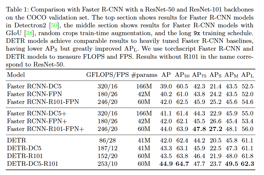
ImageNet-pretrained ResNet을 backbone으로 사용하고, Faster R-CNN과 비교했을 때 계산량이 비슷하며 성능도 동등하거나 그 이상으로 나옵니다.

4.2 Ablation

Number of encoder layers

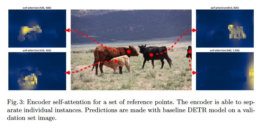
encoding layer의 수를 조절하여 image의 global self-attention 효과를 볼 수 있습니다. encode layer을 없애면 AP가 -3.9%p 하락하며, 크기가 큰 object에 대해서는 -6.0%p 하락합니다. 논문의 저자들은 encoder가 global scene reasoning(?) 과정을 통해 서로 엉켜있는 물체들의 정보들을 분리해낼 수 있다고 합니다.

위의 사진은 마지막 encode layer의 attention을 시각화 한 것입니다.

Number of decoder layers

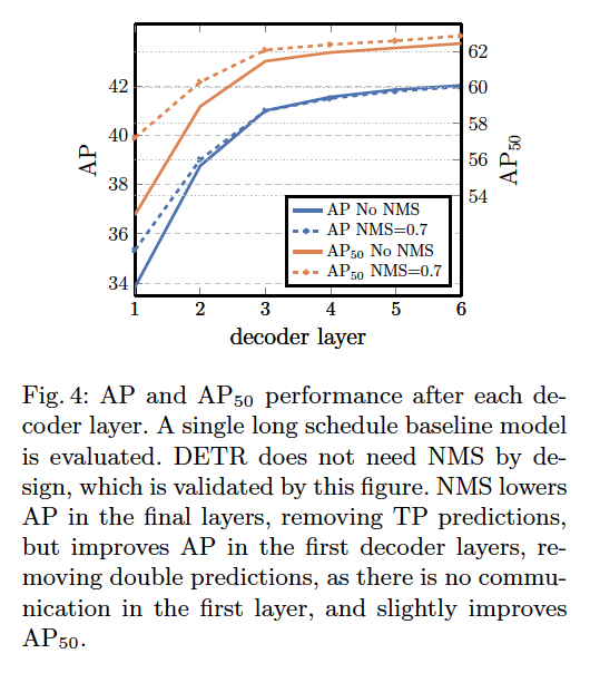
첫번째 decode layer의 output과 마지막 decode layer의 output을 비교했을 때, AP와 AP$_{50}$이 각각 +8.2/+9.5%p만큼 증가했습니다. 첫 layer의 output은 한 object에 대한 중복된 값들이 많아, 추가적으로 NMS 과정을 통해 후처리를 해주었습니다. 이는 decoder의 self-attention 방식이 output간의 cross-correlation을 계산해 중복된 값을 제거해 준다는 의미입니다.

Importance of FFN

Transformer 안의 FFN을 제거하면 파라미터 수를 41.3M -> 28.7M으로 줄이지만, 성능도 -2.3%p만큼 줄어듭니다.

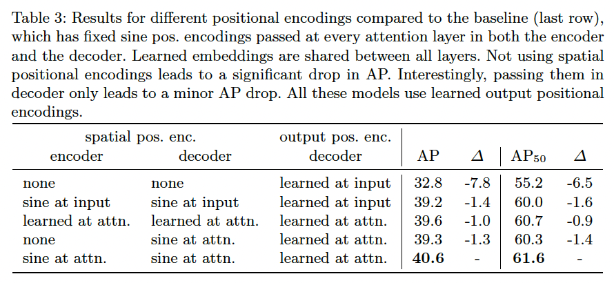
Importance of positional encodings

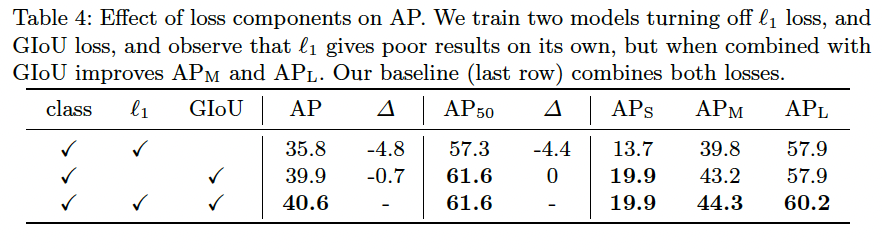
Loss ablations

4.3 Analysis

Decoder output slot analysis

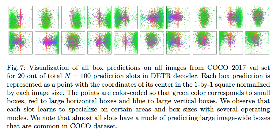
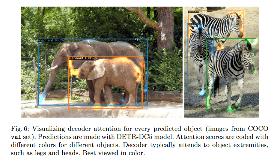
위의 그림은 COCO 2017 val set에 대한 decoder을 통한 box prediction을 시각화한 이미지이다. 초록색 점은 small box, 빨간 점은 큰 horizontal box, 파란 점은 큰 vertical box를 나타낸다. 각각의 slot이 box의 모양과 크기에 따라 서로 다른 특정 구역에 집중하는 것을 볼 수 있다.

Generalization to unseen numbers of instances

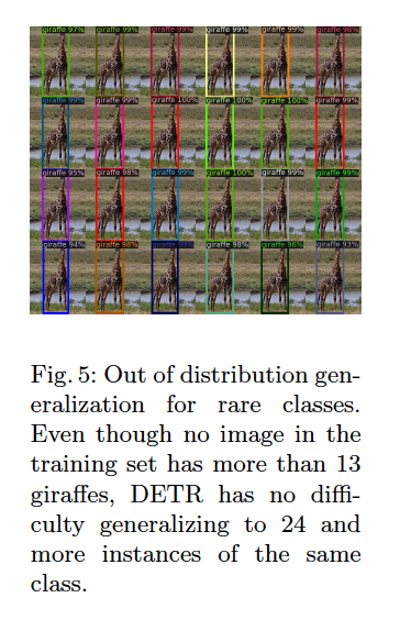
한 이미지 안에 instance의 갯수가 많은 케이스가 training set에는 없지만, 위의 그림 (기린 24마리) 과 같이 prediction은 잘 진행되는 것을 볼 수 있다. object query 각각에 strong class-specialization이 없다는 것을 볼 수 있다(?).

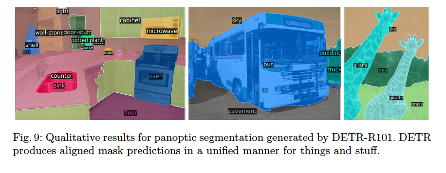
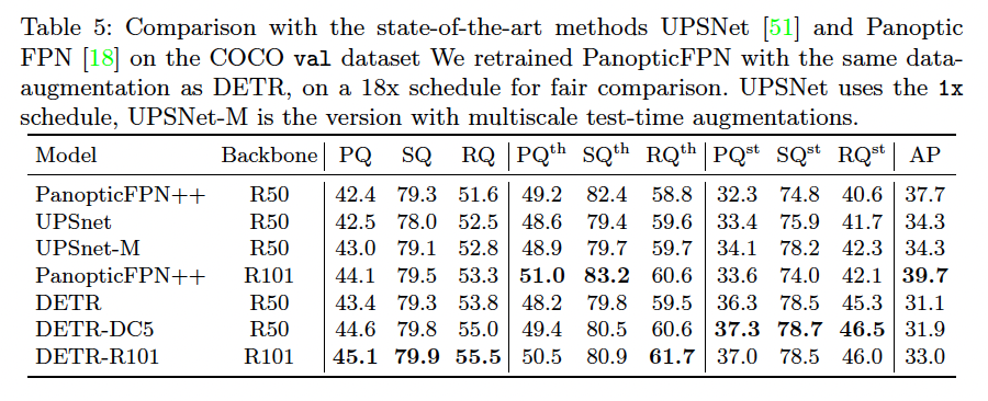
4.4 DETR for panoptic segmentation

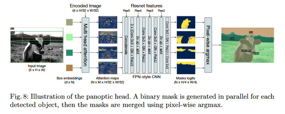
Panoptic segmentation은 주로 object detection 모델을 베이스로 삼아 진행합니다. (Faster R-CNN -> Mask R-CNN). DETR도 유사하게 decoder output을 변형해 panoptic segmentation 결과를 얻을 수 있습니다.

---

Result / Thinking

ViT / Swin과 다르게 CNN과 Transformer을 함께 사용해 모델을 구성합니다. subimage를 마치 NLP의 word와 비슷하게 해석한 ViT와는 다르게, CNN을 거친 feature map에 Transformer을 적용합니다. Segmentation분야에서 CNN과 Transformer을 합친 모델 관련된 논문을 찾아 비교해 보면 좋을 것 같습니다.

CNN을 통한 local info + Transformer을 통한 global info를 통합한 것으로 보입니다.

또한 set prediction task를 정의하고 cost를 설정해 비슷한 prediction을 제거해 후처리 없이 end-to-end 학습이 가능하다는 것 입니다.

---

Reference

https://herbwood.tistory.com/26